Evolutionary Painting
Preface
The purpose of this document is to serve me as notes and is not meant to be taken as exhaustive or a fully fledged blog post.
Introduction
In 2008 Roger Johansson released a blog post about replicating the Mona Lisa painting with only 50 semitransparent polygons: Genetic Programming: Evolution of Mona Lisa. Since then, it has served as a rite of passage and a fun project to undertake when working on genetic algorithms.
However I wanted to go further and given we were in the year 2021 when I started the project: could we actually generate a full blown painting given a target image?
This seem feasible and a quick search confirmed it with two people having had similar ideas:
- Talk from Anastasia Opara - Rust for Artists. Art for Rustaceans. — RustFest Global 2020 and the associated git repository Genetic Drawing
- Article Procedural Paintings with Genetic Evolution Algorithm from Shahriar Shahrabi and the associated git repository Procedural Painting
I did get it working and moved onto other things. However I always wanted to get back to it, clean it up and evaluate some of its properties or claims. Here are some of the notes resulting from that work.
Initial implementation
As mentioned in the Overview, we want to model our painting as a series of brush strokes. While it is certainly possible to evolve whole paintings at once, given that paintings can have thousands of strokes, it can become a space too large to explore meaningfully in a realistic amount of time.
Since the paint strokes are additive, we can work on a subset of the strokes at a time and make our way to the final painting that way. This means we will define iterations of N strokes that we will optimize and then move on to the next iteration until satisfied or some limits are reached (ex: number of strokes, fitness reached or unable to improve, etc.). Thus each iteration will run a full genetic algorithm optimization on the current subset of strokes and will build upon the generated painting from the previous iteration.

In addition, since we are going to do some image processing, we will use:
Chromosomes
The chromosomes need to allow the expression of multiple brush strokes. But how is a brush stroke defined? Each one will require the following information:
- Position (x, y)
- Color (r, g, b)
- Angle
- Size
- Which stroke style
This is a total of 8 parameters for each brush stroke.
For a given iteration of N strokes, it means we will be optimizing \$N * 8\$ parameters.
Brushes
The reason we have a parameter to select the style of the brush stroke, is that if we use the same style for each stroke, this will create a visually unappealing painting. The human eye will catch very quickly that each stroke is strictly identical and thus would look quite odd. To avoid such monotony, we will introduce variety in the strokes by preparing enough different strokes so as to not stand out as much.
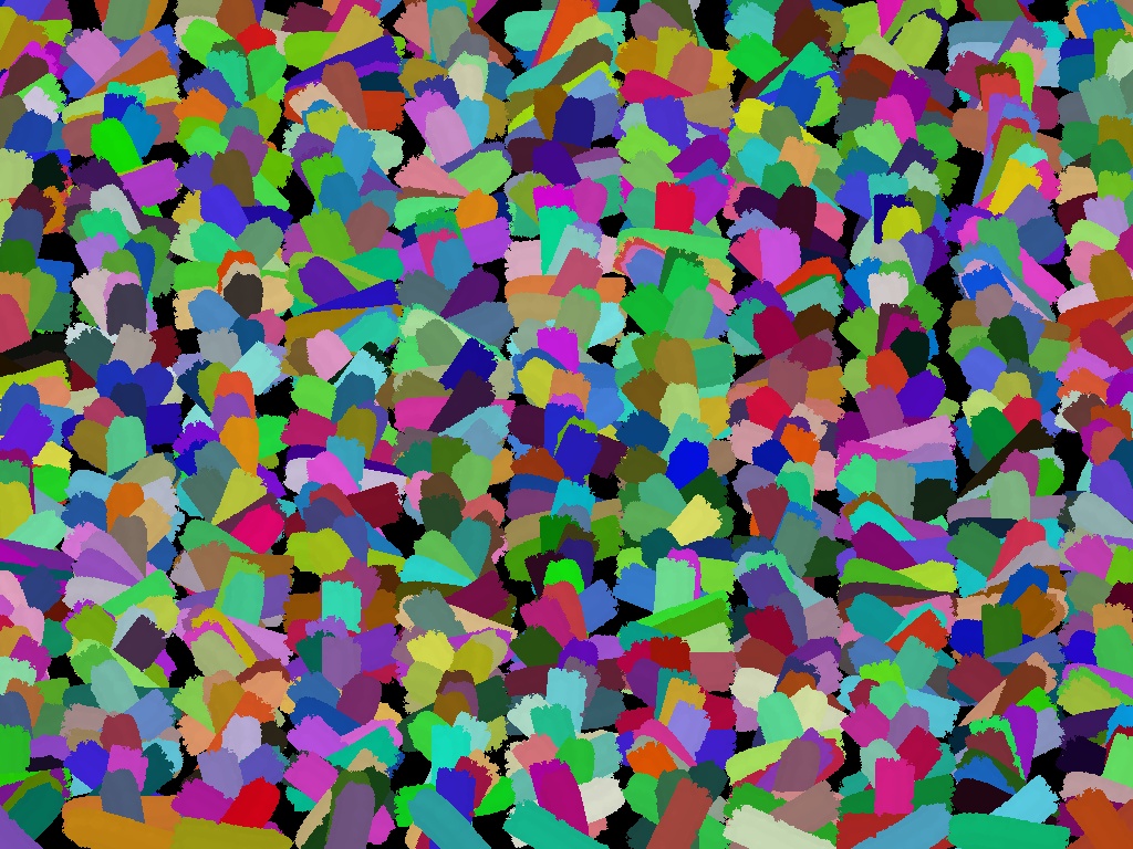
Here is an example where strokes are generated with random position, orientation and color but with the exact same style. We can observe how the human eye latches on the similar look of each stroke and how it can make it too fake if it was used in a real painting.
Different brushes were created with the help of Krita:
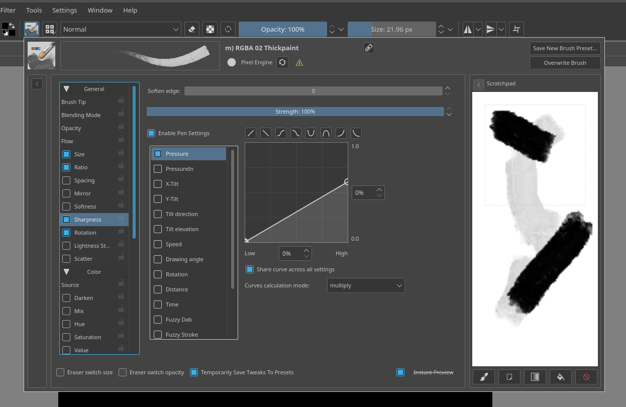
Their size being a parameter of the chromosome, it can be a value between 0 and 1, which is the scale factor of the brush pictures passed to the program.
Fitness
There remains the problem of defining a fitness function since it will guide the evolution and what constitutes the best brush stroke at a given stage. While there are many considerations and options, we will start by a simple sum of the differences of the pixels between the target image and the generated painting using their RGB values.
RGB colors are used for their simplicity and to get us started, however we need to be mindful they aren’t in a linear color space, which may not be perfect when doing a difference between rgb values.
Benchmark
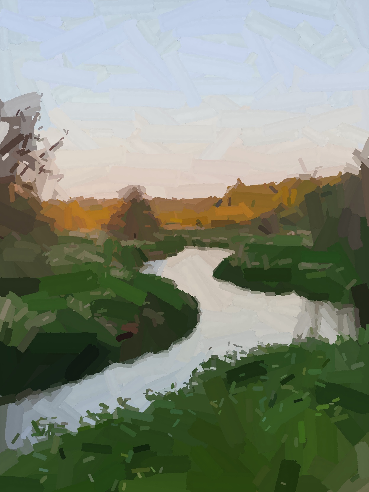
We will need a set of images we want to paint to validate the results and understand better when and why specific cases work the way they do and whether or not the results are satisfying or not.
I may eventually add a more rigorous set of images based on specific features (ex: related to frequencies, gradient, color space, etc.) but since it’s supposed to be a fun project, I have settled on a few pictures.
Through their gradients, colors and themes, all these pictures underline a different aspect and will challenge the program in different ways.
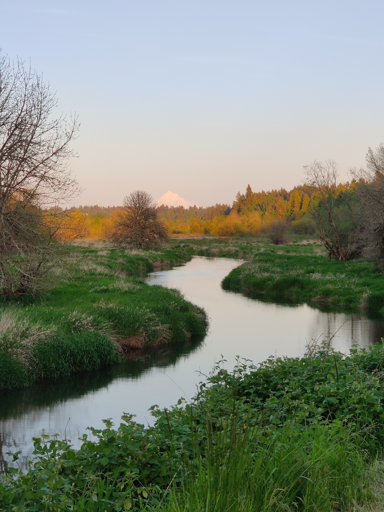


These include photos from Unsplash by Vladislav Nahorny for the ferris wheel, Georg Eiermann for the jellyfish, and sahil muhammed for the close up fly. The others are from me.
Performance aspects
Let’s take a step back and assume the following:
- We have \$I\$ iterations
- Each iteration optimizes \$N\$ brush strokes
- We have a population size of \$P\$ individuals, each encoding a series of strokes for a given iteration
- The combination process of the genetic algorithm will generate \$2\$ children
- Each iteration will go through \$G\$ generations
That means we should expect to evaluate \$2 xx I xx P xx G\$ paintings total and that the final painting will contain \$N xx I\$ brush strokes.
| Number of iterations - I | Number of brush strokes at each iteration - N | Population size - P | Generations for each iteration - G | Total number of strokes | Number of paintings evaluated for each iteration | Number of paintings evaluated - Total |
|---|---|---|---|---|---|---|
| 1 | 10 | 10 | 100 | 10 | 2,000 | 2,000 |
| 100 | 10 | 100 | 100 | 1,000 | 20,000 | 2,000,000 |
| 100 | 10 | 10 | 100 | 1,000 | 2,000 | 200,000 |
| 100 | 10 | 300 | 1,000 | 1,000 | 600,000 | 60,000,000 |
| 100 | 10 | 300 | 1,500 | 1,000 | 900,000 | 90,000,000 |
| 200 | 10 | 300 | 1,500 | 2,000 | 900,000 | 180,000,000 |
| 300 | 10 | 300 | 1,500 | 3,000 | 900,000 | 270,000,000 |
| 400 | 10 | 300 | 1,500 | 4,000 | 900,000 | 360,000,000 |
| 500 | 10 | 300 | 1,500 | 5,000 | 900,000 | 450,000,000 |
We can observe that while the relationship between the parameters is linear, their combination does end up requiring quite a bit of paintings to evaluate and I expect it to dominate the total runtime.
This gets more complicated once we factor in the painting size.
If we put in equation the speed at which we need to evaluate an individual painting, we end up with \$"Evaluation time for a single individual in second" = "Number of paintings" / "Allocated time in second"\$. From the table above, we can infer we will have to evaluate tens, if not hundreds, of millions of paintings. And if we want that to happen in a matter of hours, that implies evaluating a painting cannot take longer than a few hundreds microsecond.
Moving the expensive computations to GPU
Initial implementation on CPU
I started the implementation of that project by generating the painting with OpenCV on the CPU. This has enabled me to validate my algorithms and get up and running quickly. However the computations were unbearably low.
Experimentally, I obtained the following performance:
- For a 300x400 painting, it takes ~2.83 millisecond for each individual
- For a 1024x768 painting, it takes ~1.467 second for each individual
Note: Each iteration logs information about the generations in a separate log file. The methodology for the timing measurements is to look at the time difference across the timestamps of the CSV log files and to normalize it by the number of generations and individuals. This implies any multi-threading considerations are already baked into them and thus the performance is not equivalent to computing a single painting on a single core of a CPU.
If we were to plug the numbers for a 1024x768 painting in the previous table, that would give us:
| Number of iterations - I | Population size - P | Generations for each iteration - G | Number of paintings evaluated for each iteration | Number of paintings evaluated - Total | Computation time for each iteration (minute) | Total computation time (hour) | Total computation time (day) |
|---|---|---|---|---|---|---|---|
| 1 | 10 | 100 | 2,000 | 2,000 | 0.162 | 0.0027 | 0.000113 |
| 100 | 100 | 100 | 20,000 | 2,000,000 | 1.62 | 2.71 | 0.113 |
| 100 | 10 | 100 | 2,000 | 200,000 | 0.162 | 0.27 | 0.0113 |
| 100 | 300 | 1,000 | 600,000 | 60,000,000 | 48.75 | 81.24 | 3.39 |
| 100 | 300 | 1,500 | 900,000 | 90,000,000 | 73.12 | 121.86 | 5.08 |
| 200 | 300 | 1,500 | 900,000 | 180,000,000 | 73.12 | 243.73 | 10.16 |
| 300 | 300 | 1,500 | 900,000 | 270,000,000 | 73.12 | 365.59 | 15.23 |
| 400 | 300 | 1,500 | 900,000 | 360,000,000 | 73.12 | 487.45 | 20.31 |
| 500 | 300 | 1,500 | 900,000 | 450,000,000 | 73.12 | 609.32 | 25.39 |
In addition to making it difficult to quickly explore and iterate on ideas, this means any sensibly detailed painting or with size large enough to be printed would take weeks to compute.
Implementing on GPU
Luckily, Genetics4j supports GPU based computations through its gpu module with OpenCL. The required steps amount to:
- Add a dependency on the gpu module from Genetics4j in the project
- Use GPUEAConfiguration and GPUEAExecutionContext instead of the regular EAConfiguration and EAExecutionContext
- Use GPUEASystemFactory instead of the regular EASystemFactory
- Update the GPUEAConfiguration with:
- Add information about the OpenCL program, its source, parameters, available kernels
- Update the fitness computation with either a SingleKernelFitness if there is a single OpenCL kernel to execute or a MultiStageFitness if multiple OpenCL kernels need to be chained. Be aware they do provide some facilities to reuse pieces of data and to avoid unnecessary back and forth between the GPU and the host
GPUs are organized and work differently from a regular CPU. They have many cores which follow the same flow. As such, the initial approach was to batch the individuals to process and use a single kernel which would work on each pixel of the generated painting separately and would have the following steps:
- On the GPU side, for each individual in the batch, we apply the brush strokes if applicable. We then do a difference between the the target image and the painting and store the result in an array to send back to the CPU
- On the CPU side, when generating the final fitness score, we do a sum of all these differences
This worked great and improved the performance quite a bit. However there were two issues:
- Each brush stroke has a specific rotation, scale and position. Since the OpenCL kernel was working at the pixel level, that means the same transformation matrix was computed for each pixel to see if it was within a brush stroke. Therefore it makes sense to extract this into its own compute kernel and store the resulting transformation matrix in the GPU memory. Further kernels can look up that information
- Doing the sum of all the differences on the CPU is inefficient as it means transferring a lot of data (\$"Batch Size xx Width xx Height\$) and then do the sums on the CPU when a GPU would be incredibly more efficient at it. So that also ended up being improved with doing partial sums as much as possible on the GPU and doing a final aggregation on the CPU with a greatly reduced data size
In the end, experimentally, for a 1248x1664 painting, it takes ~308 microsecond for each individual. Going through the same exercise as before with the previous table:
| Number of iterations - I | Population size - P | Generations for each iteration - G | Number of paintings evaluated for each iteration | Number of paintings evaluated - Total | Computation time for each iteration (minute) | Total computation time (hour) | Total computation time (day) |
|---|---|---|---|---|---|---|---|
| 1 | 10 | 100 | 2,000 | 2,000 | 0.01 | 0.00017 | Too small |
| 100 | 100 | 100 | 20,000 | 2,000,000 | 0.103 | 0.171 | 0.007 |
| 100 | 10 | 100 | 2,000 | 200,000 | 0.01 | 0.017 | 0.0007 |
| 100 | 300 | 1,000 | 600,000 | 60,000,000 | 3.084 | 5.14 | 0.214 |
| 100 | 300 | 1,500 | 900,000 | 90,000,000 | 4.626 | 7.71 | 0.321 |
| 200 | 300 | 1,500 | 900,000 | 180,000,000 | 4.626 | 15.4 | 0.642 |
| 300 | 300 | 1,500 | 900,000 | 270,000,000 | 4.626 | 23.13 | 0.964 |
| 400 | 300 | 1,500 | 900,000 | 360,000,000 | 4.626 | 30.84 | 1.285 |
| 500 | 300 | 1,500 | 900,000 | 450,000,000 | 4.626 | 38.55 | 1.606 |
Even with \$(1248 xx 1664)/(1024 xx 768) = 2.64\$ times more pixels, we expect and observe a dramatic improvement in performance. It’s amazing to see what would take almost 3 days and a half on a multi-core CPU would now only take 5 hours with a GPU. And as we go higher in the complexity, 50 days worth of CPU computations on a multi-core CPU would take slightly over 3 days.
I could continue with further GPU related optimizations, but this has become good enough for the purpose of this project.
Further improvements
A popular stopping criterion for evolutionary algorithms is to employ an adaptive method that will stop if we do not observe any improvement in the fitness for \$N\$ generations. Fortunately, Genetics4j provides support for that exact method with the termination factory Terminations.ofStableFitness.
This looks promising and we will want to validate that it is an appropriate method in this project. As part of this process, we will want to answer the following questions:
- How early would it stop for different values of that stability criterion?
- Is the loss of potential fitness improvement acceptable? Had we been through all the generations, would we have a fantastically improved fitness?
To answer these questions, I did run an experiment where I compute a painting for 1500 generations and then would look at the impact had we used that adaptive method with different parameters. Doing so across multiple runs to gather more robust data and across different values for the stability criterion so we can compare and contrast.
After running that experiment, we can derive some interesting information. Starting with the graphs about the stopping point:
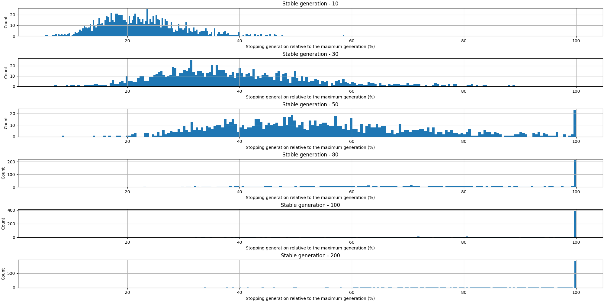
That first plot is expected as it is normal to observe that shorter values for the adaptive stopping result in the evolution stopping earlier. Let’s turn our attention to the stopping points over time:
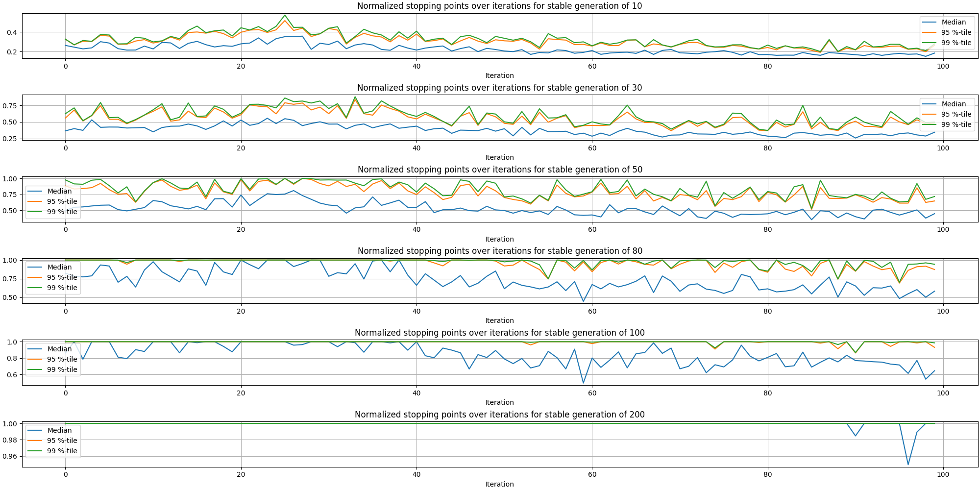
We can observe it is more likely to stop the evolution sooner at later stages of the painting than at the beginning. This makes sense since earlier stages have more opportunities for improvement than the later ones. And now, here is a plot putting in relation the stopping generation (normalized) with the adaptive stopping parameter:
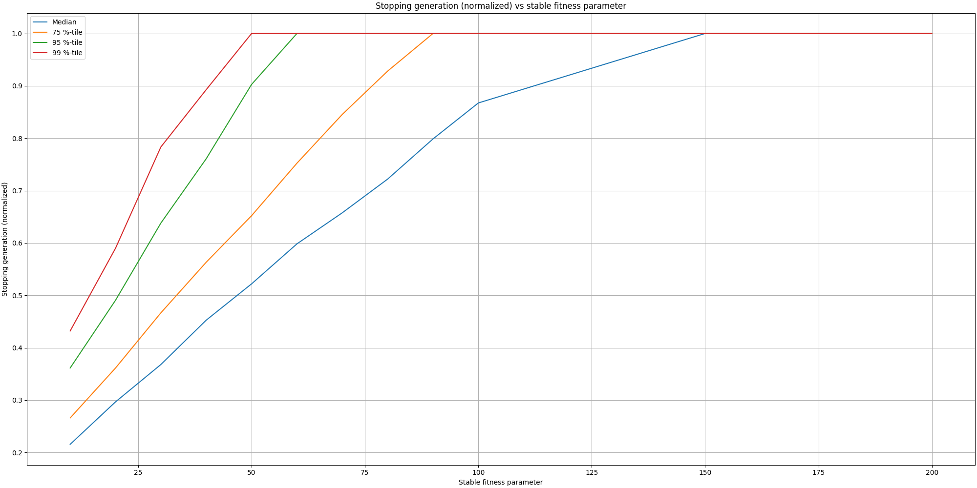
This is quite interesting to see how it can save many generations from being computed. If we take a parameter of 50 stable generations, we can observe that half of the time it would stop half way! This is great to see we can save a lot of computation and thus time, but we also need to validate we aren’t missing too much on the fitness. So let’s start by looking at the histogram of losses based on the adaptive stopping parameter:
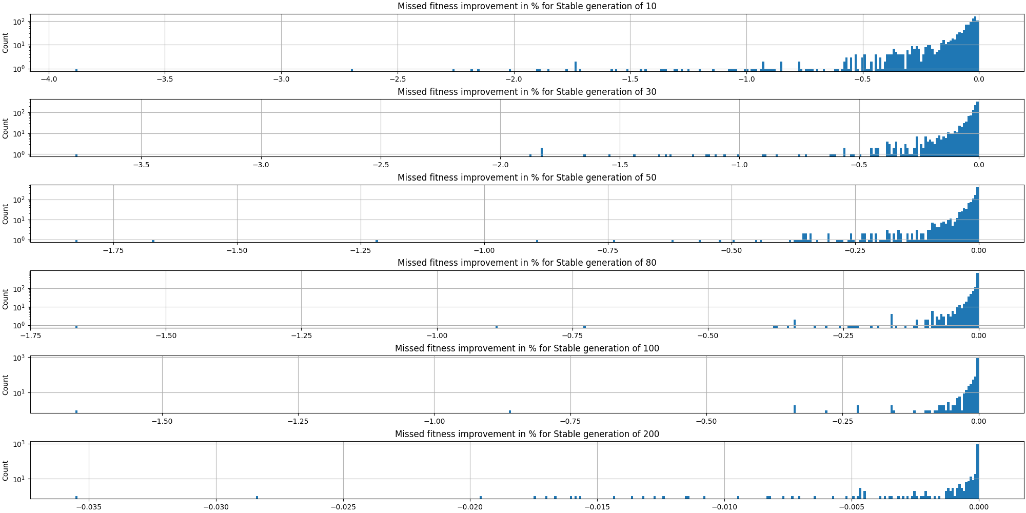
The first thing we note is how little is the loss of opportunity in fitness, even for low values for the adaptive parameter.
Let’s look at the missed fitness over time:
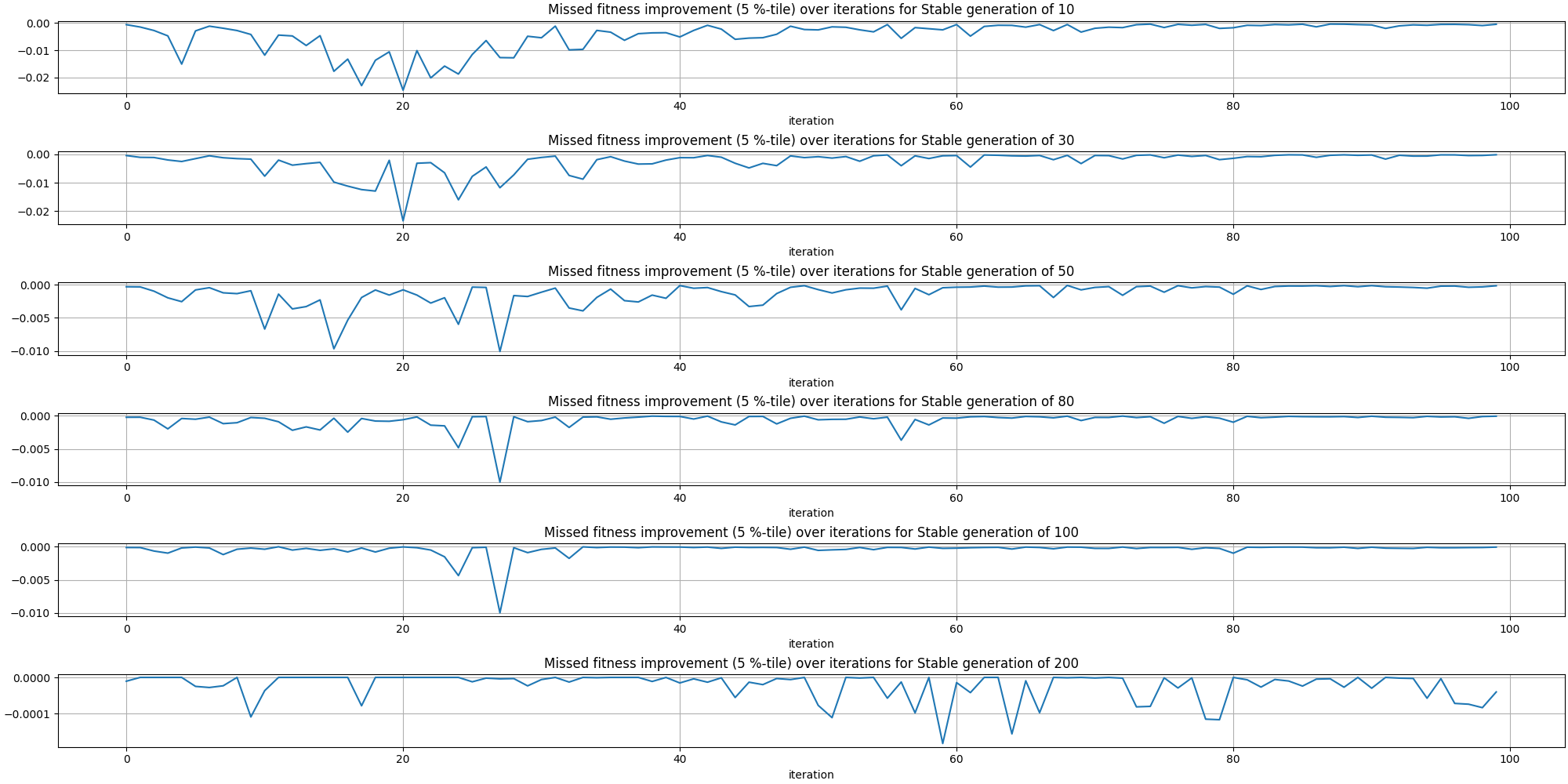
There is an interesting pattern emerging where most of the missed fitness happens early on rather than at later stages.
Finally, let’s look at the fitness loss for different values of the stable fitness parameter:
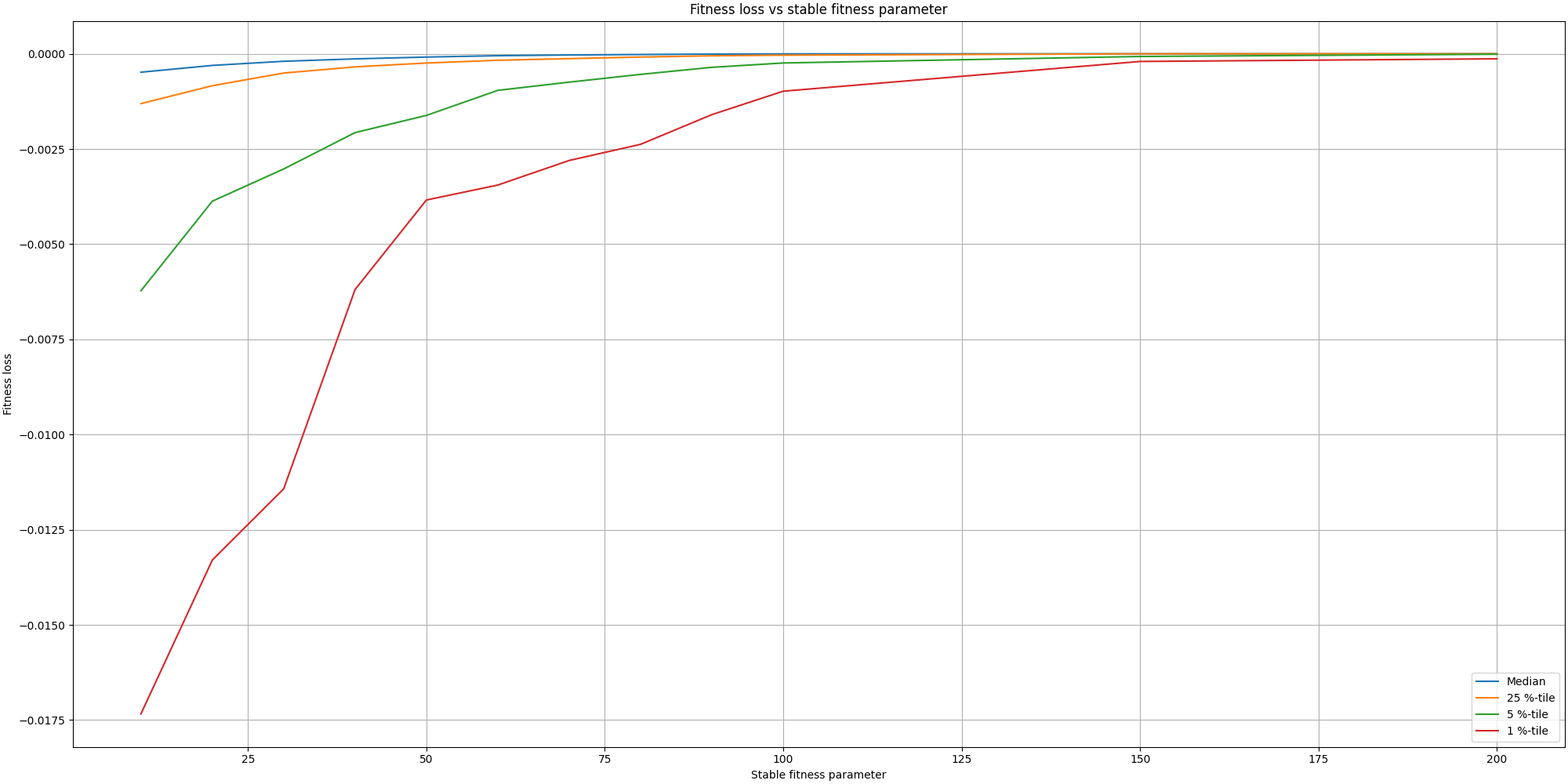
We can observe how little is the loss in most cases.
Overall the loss in quality is acceptable comparing to the large gains in time. It is also fascinating to see this small optimization having more impact than any other GPU optimization I could add.
We could take it further in the future, by optimizing the stable fitness parameter over time. As the plots above show, it has a higher chance to miss on fitness at earlier stages despite stopping later. Thus we could reduce the miss in fitness by using larger stable fitness parameters early on and then relaxing it over time.
Qualitative assessment
First results
We have looked at a lot of graphs but nothing about the produced paintings yet. So let’s look at our first painting:
This looks great, except for the parts of the painting that aren’t painted. They stand out and are problematic. However it can be explained by our current fitness function where filling blanks is not rewarded and even if "the algorithm" wanted to do so, there would be other places to paint with a better reward.
To address this issue, it means we need to incorporate such criterion into our fitness function. We also need to be mindful as to not distract the fitness function as a painter would not just try to fill out blanks first. As such, we will use the alpha component as information about whether or not a pixel has been painted before and will add a new component to the fitness in the form of \$1 + a * ("iteration"/"total iterations")^2\$, with \$a\$ being a positive constant.
Plotting it brings:
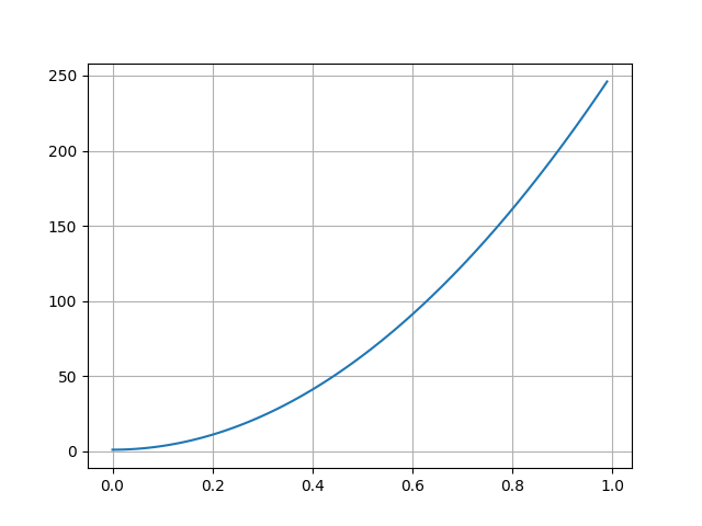
We can observe the cost of an unpainted pixel will gradually increase as time pass, with he benefit of not creating an upfront cost in filling the blanks but ensuring the algorithm will start paying more attention over time as its cost increases. In my implementation, I set a parameter that let me disable that additional cost until we have reached enough iterations.
Improved results
As we have fixed the issue with holes in our paintings, let’s start with a video walking through all the brush strokes for one of our enhanced painting:
This was produced with 100 iterations and the default parameters outlined earlier. Here is the final image:
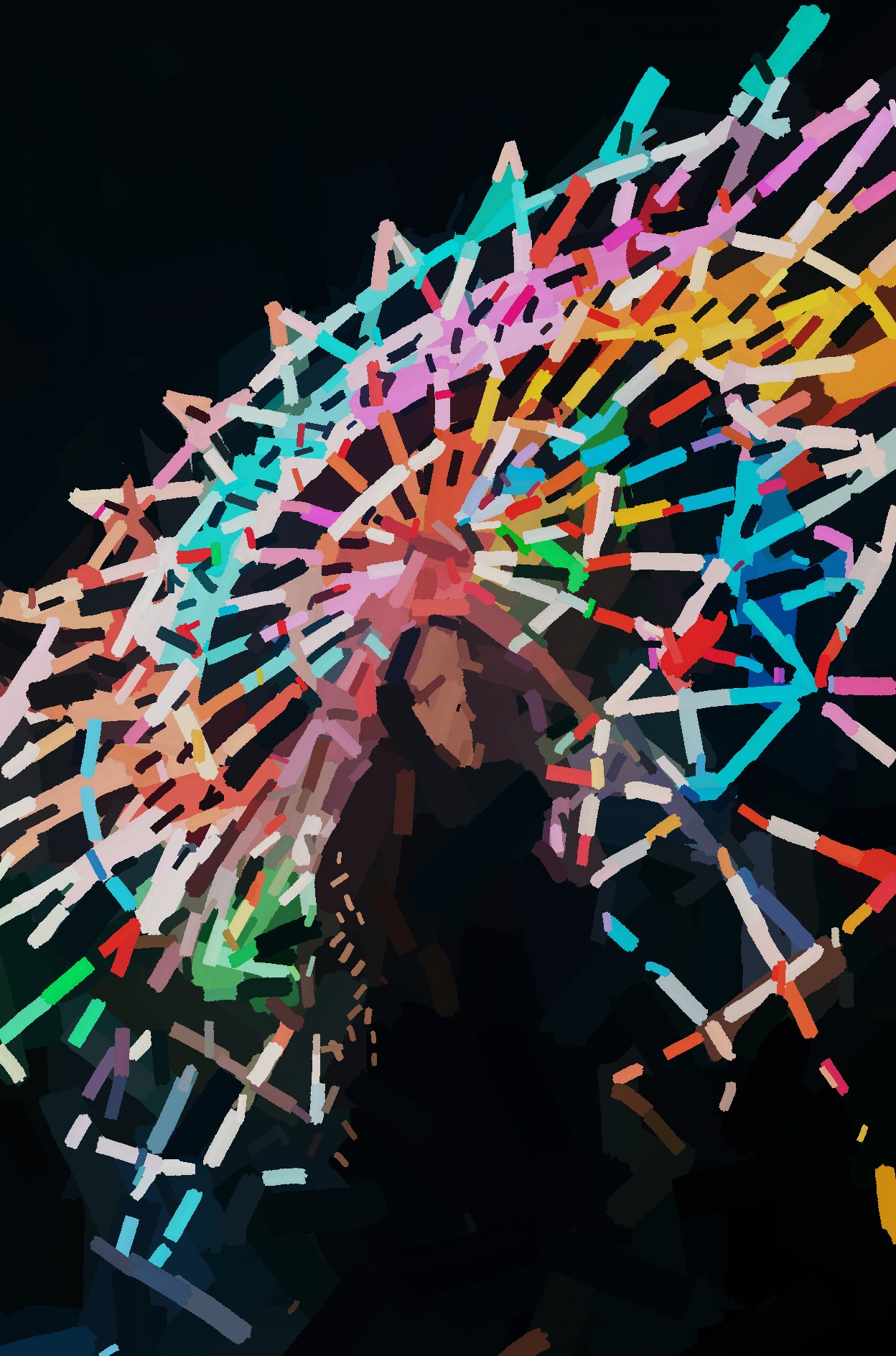
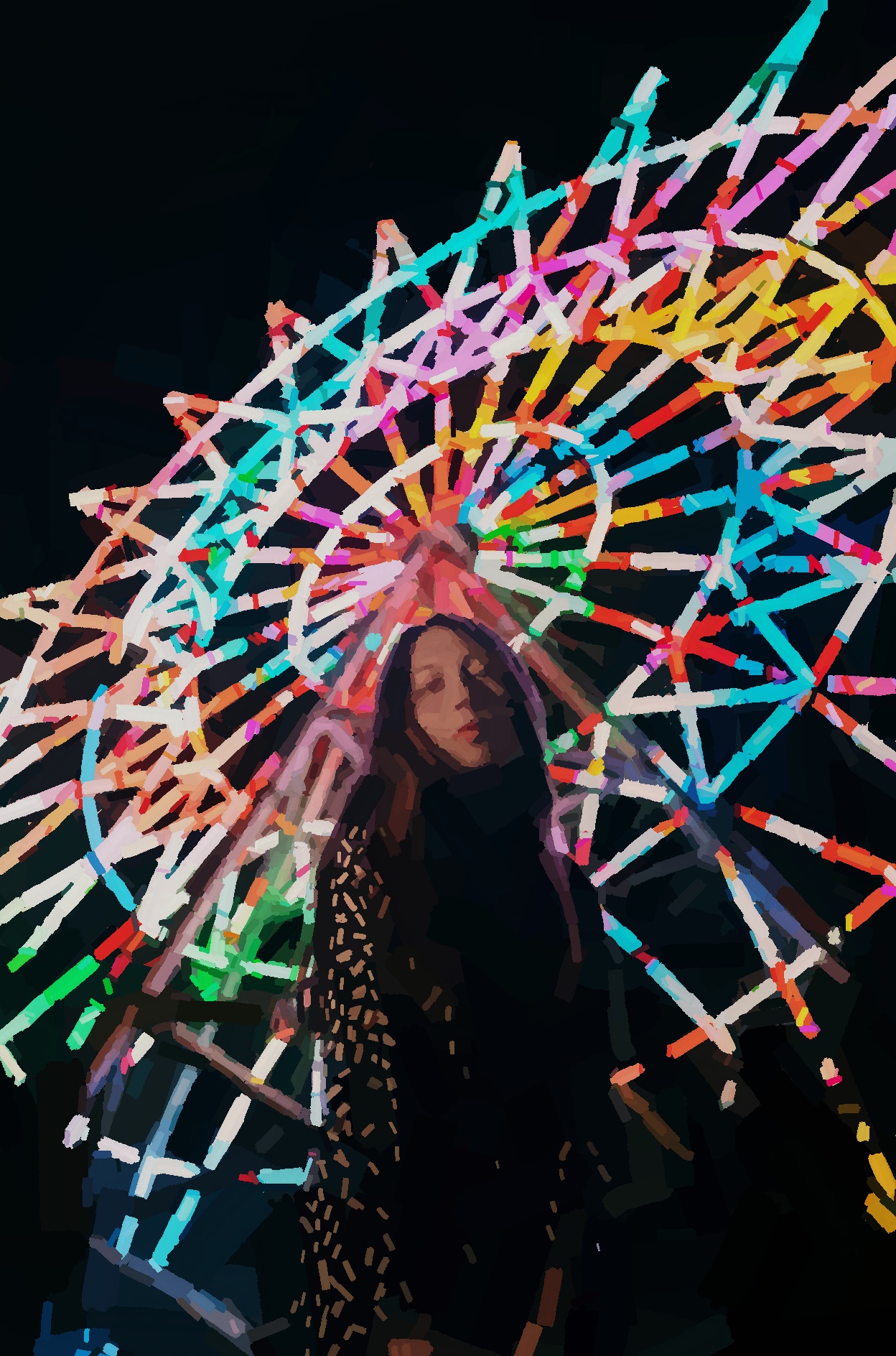
Next on our benchmark is the ferris wheel at night with a lady in front. I am including two images for comparison where the first image has run through 100 iterations while the second one, on the right, has run through 300 iterations. We can notice some interesting features, especially around the details and how the evolution did not get to finish painting the patterns on the lady’s jacket.
The painting with 300 iterations might feel too much like a copy of photography and I would expect some of the iterations in between to give a more artistic feeling.
We should also note a limitation in our fitness function. Since it only prioritizes the differences in pixel, it does not care about which areas are prioritized over others. And in this case, that would explain why the face of the lady lacks so much details in the picture on the left since the algorithm would find a better fitness by improving other areas with larger differences, such as this big brightly colored wheel.
 |
 |
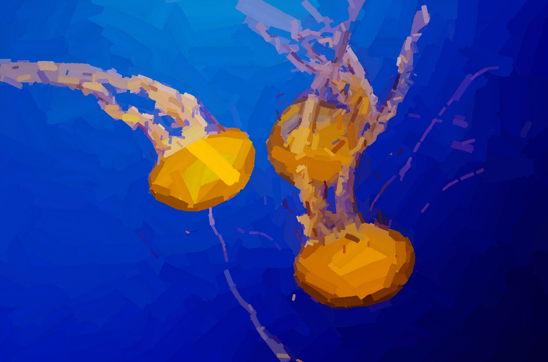
Then we have the jellyfish. The lack of details do give it some artistic sense. However the tentacles would benefit from more details
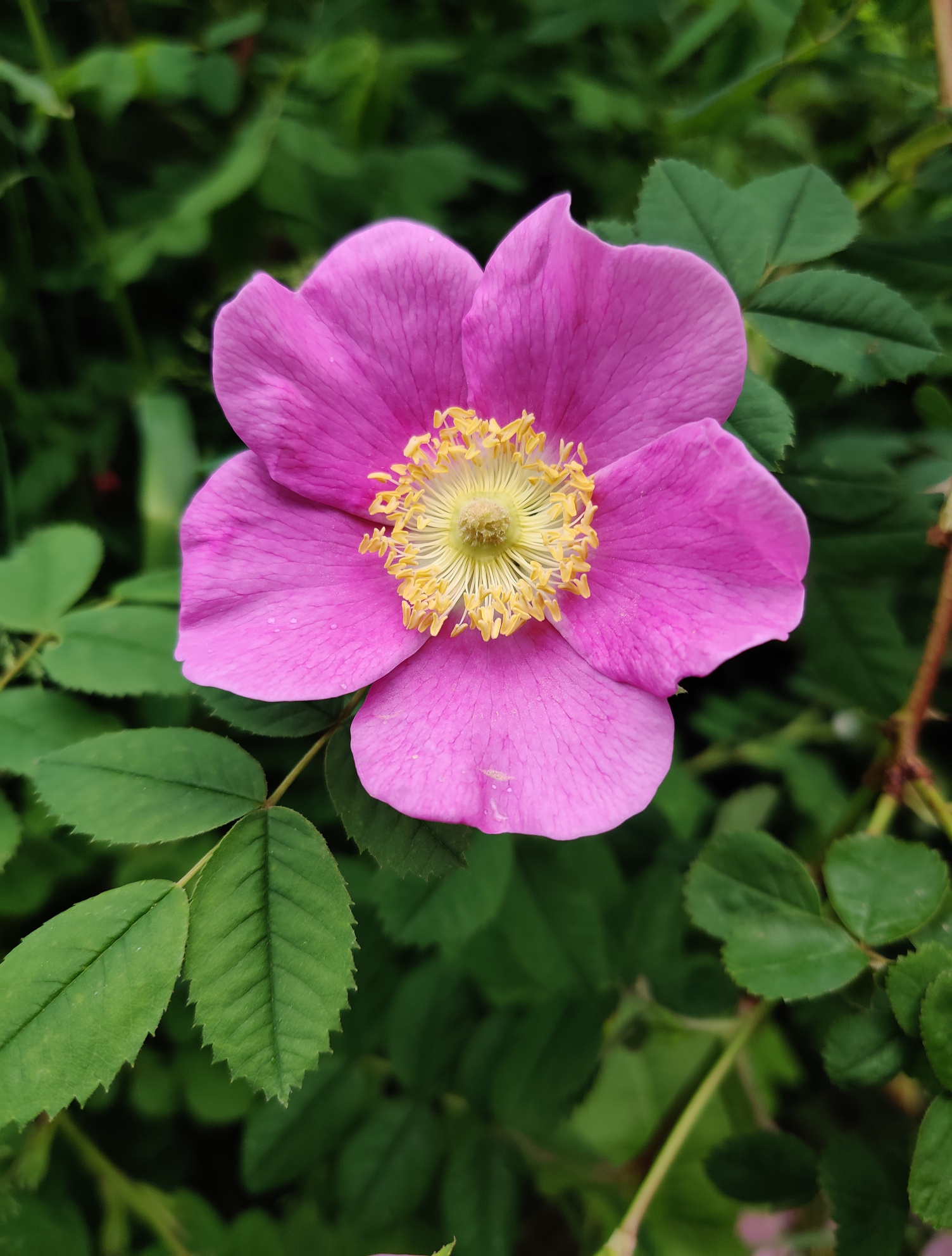
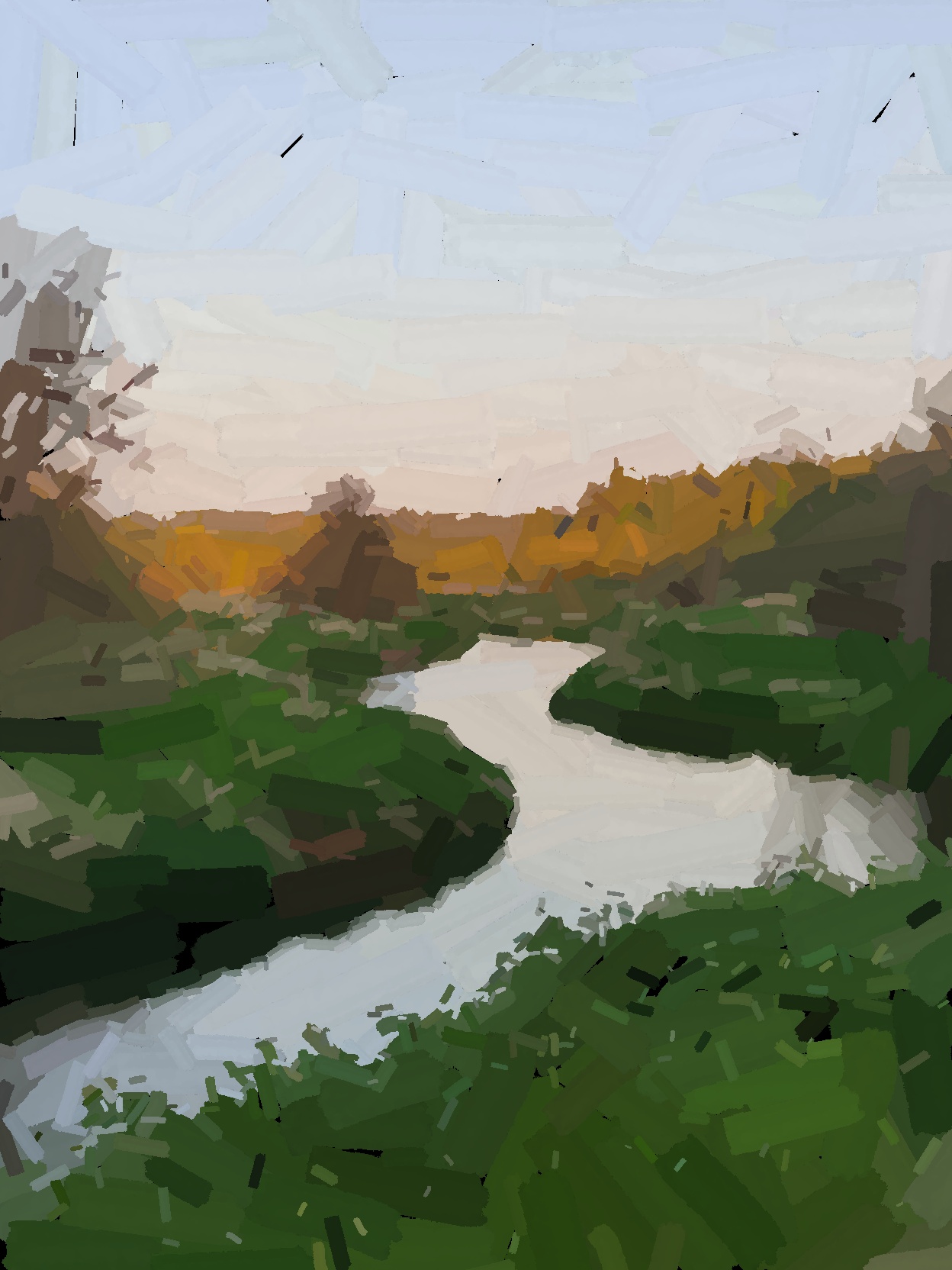
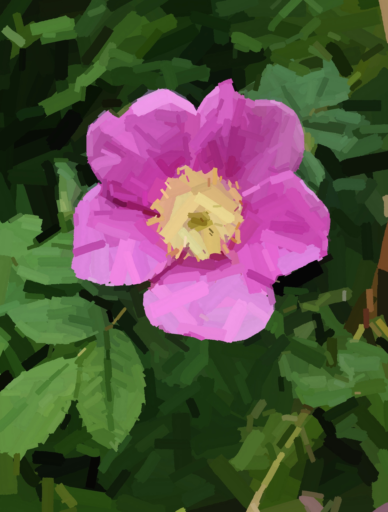
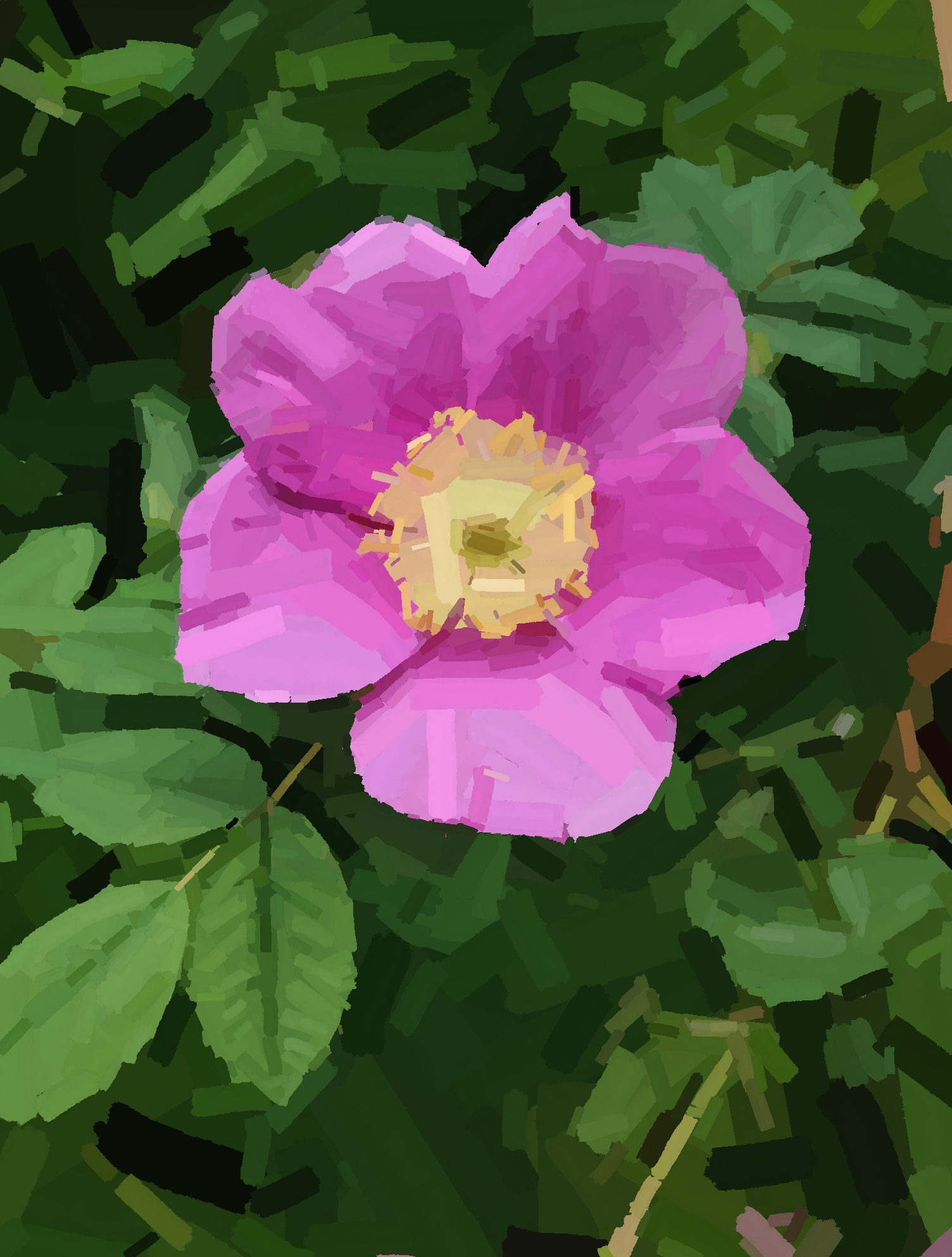
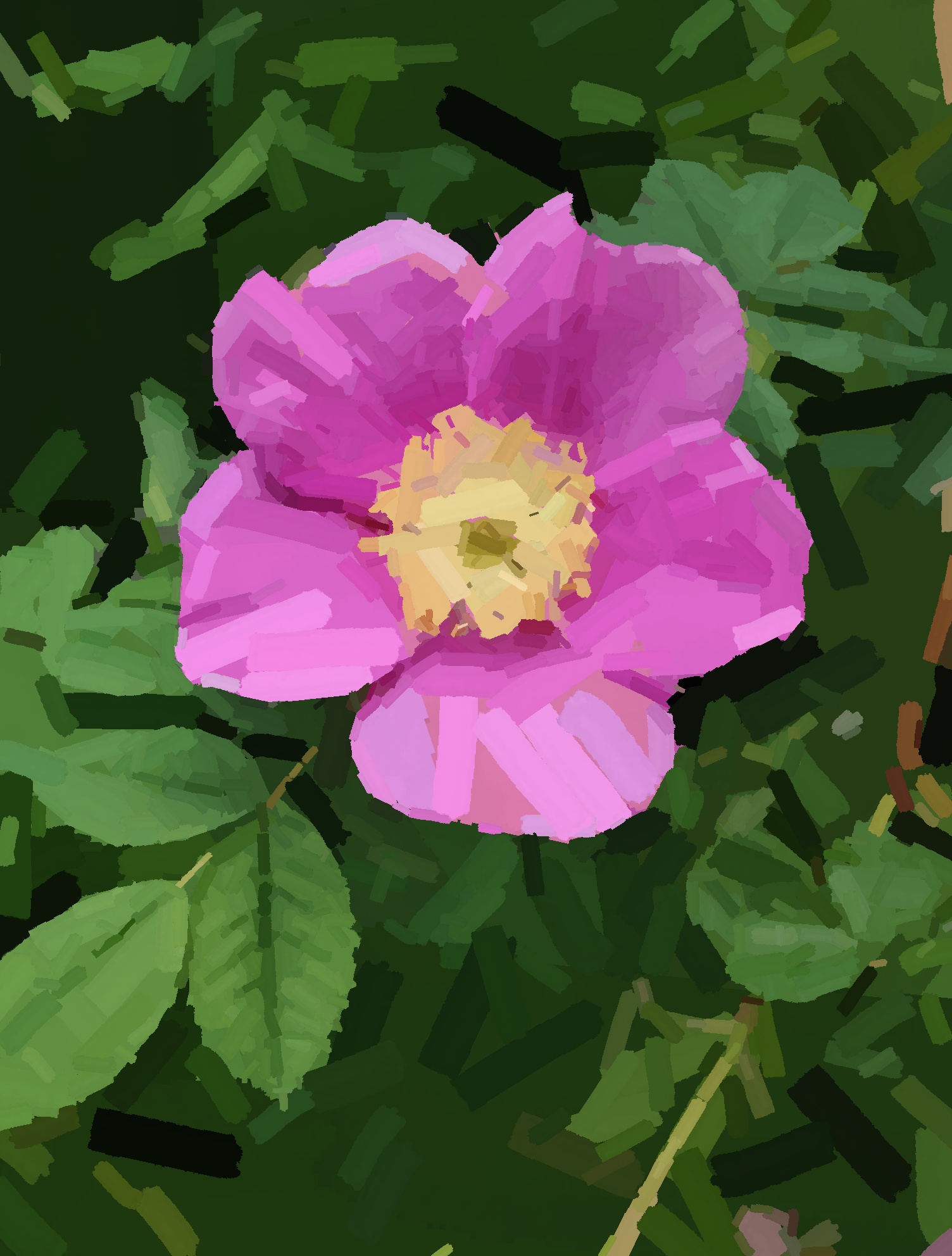
Followed by a flower from my yard
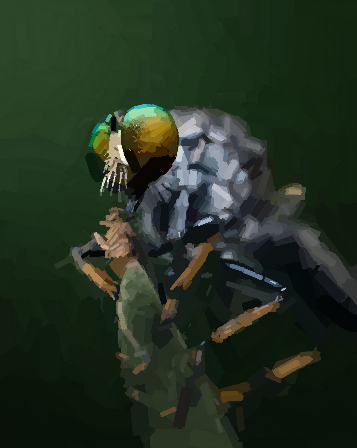
And finally we have the close up shot of an insect. It looks quite nice and represent clearly the areas in focus and out of focus. This is an especially tricky painting given the complexity of the eyes.
Improvements
Evaluating sampling from edges
Some articles described how they used edges from the original picture to guide the initial position and orientation of the strokes, especially as the iterations progress. This reflects the process of a human painter who would start with the broad strokes and focuses more and more on the details towards the end as the painting progresses. This looks quite interesting and we should put it to the test!
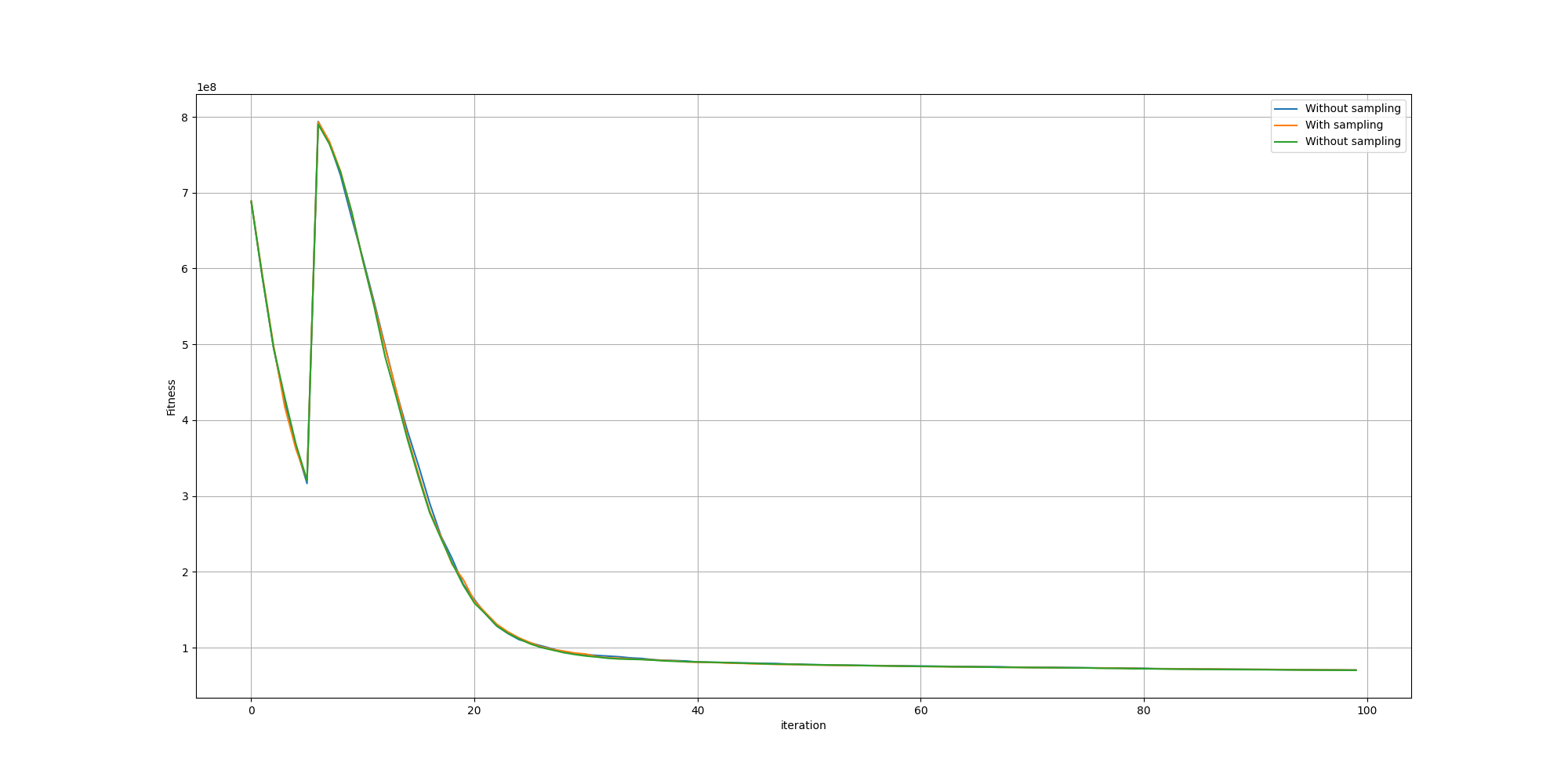
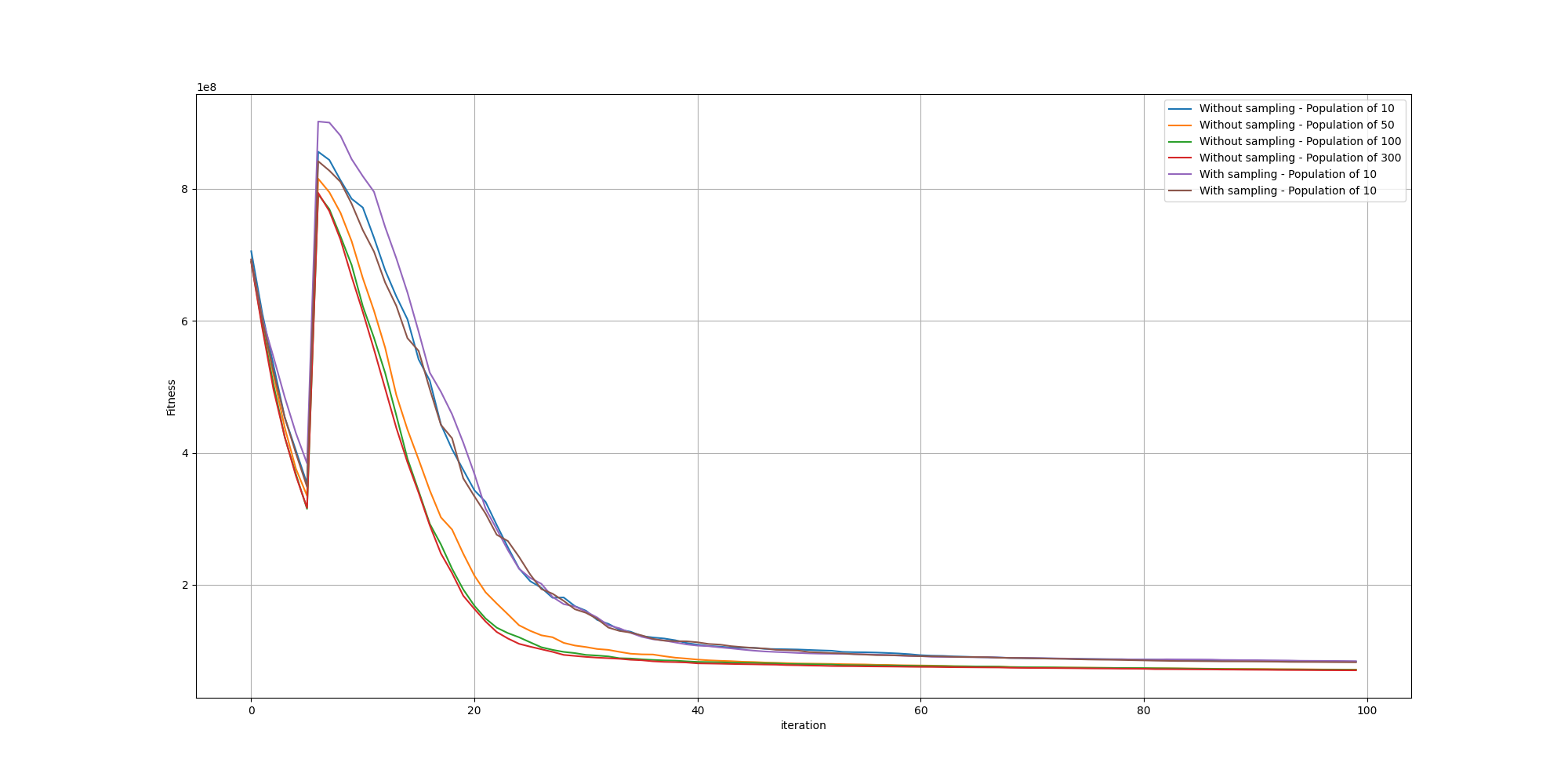
Let’s look at how the 5 percentile fitness of such paintings fare comparing to paintings without sampling:
And let’s zoom to the last iterations so we can see better:
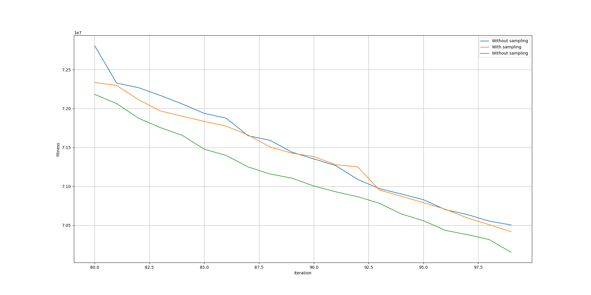
Unfortunately, we cannot observe any meaningful improvement. However one hypothesis might be that since we can leverage GPUs, we can afford larger populations and thus do not gain any advantage with the sampling method since the space of solutions will be sufficiently explored. But we can put that to the test was well by comparing the fitnesses run with different population sizes!
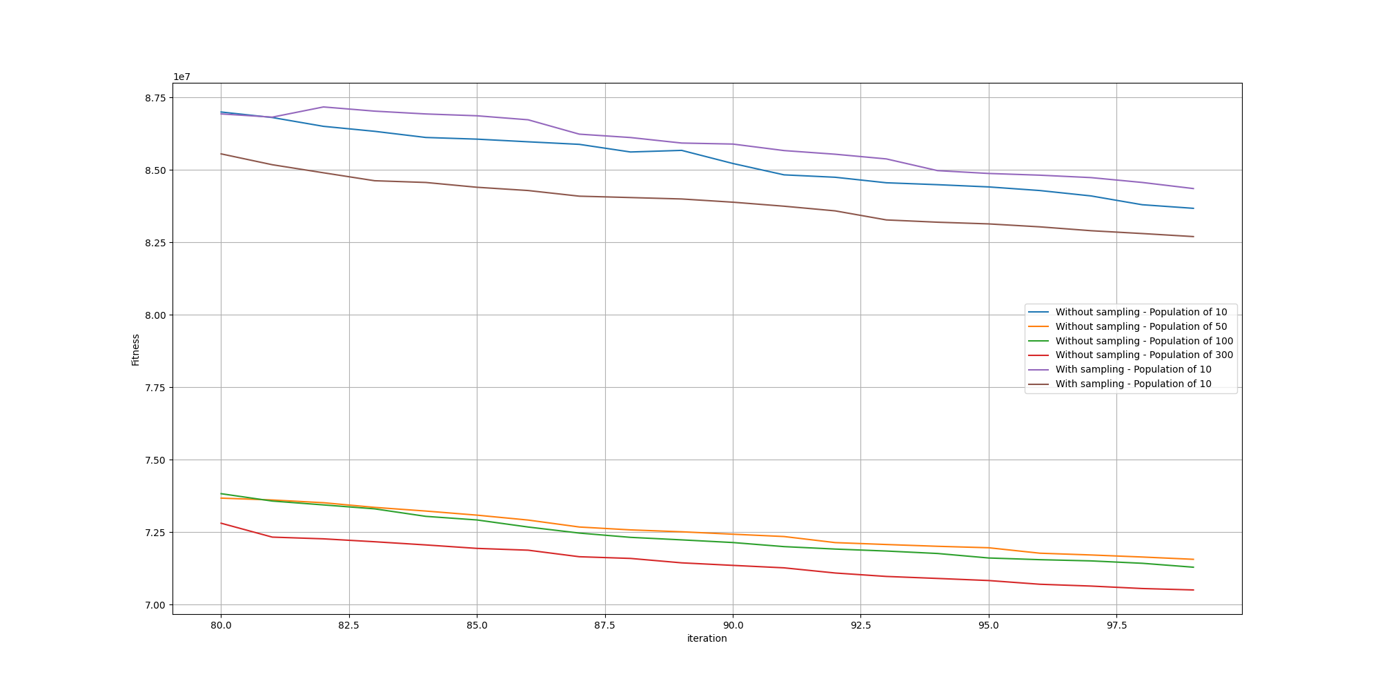
There again, we do not see any meaningful impact from the edge sampling based method. We can also observe along the way how increasing the population size improves the fitness.
However it does not mean we should discard that idea completely. It could help contribute to more natural looking paintings, but that would probably work better if integrated into the fitness.
Brush sizes
We should look into the maximum brush size and its impact on paintings. Is there an optimal size? How might we determine it?
To understand better the behavior, I did generate multiple paintings of the flower with different maximum brush sizes, starting with the default size noted as 1x to seven times the maximum size noted as 7x. In this context, using the parameter of 7x means brush strokes can have a size from 0 all the way to 7 times the default maximum size.
We can look at the resulting fitnesses:
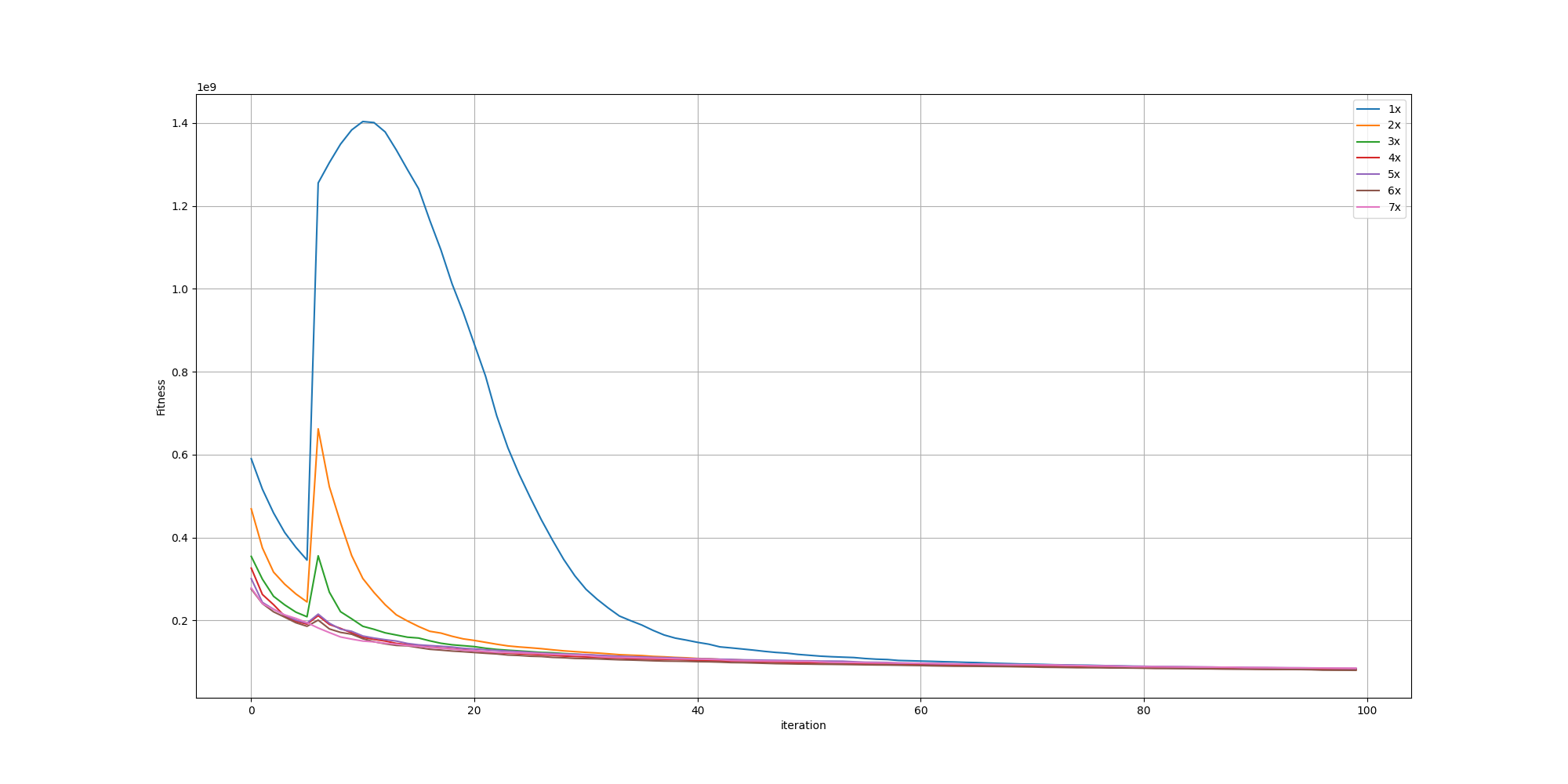
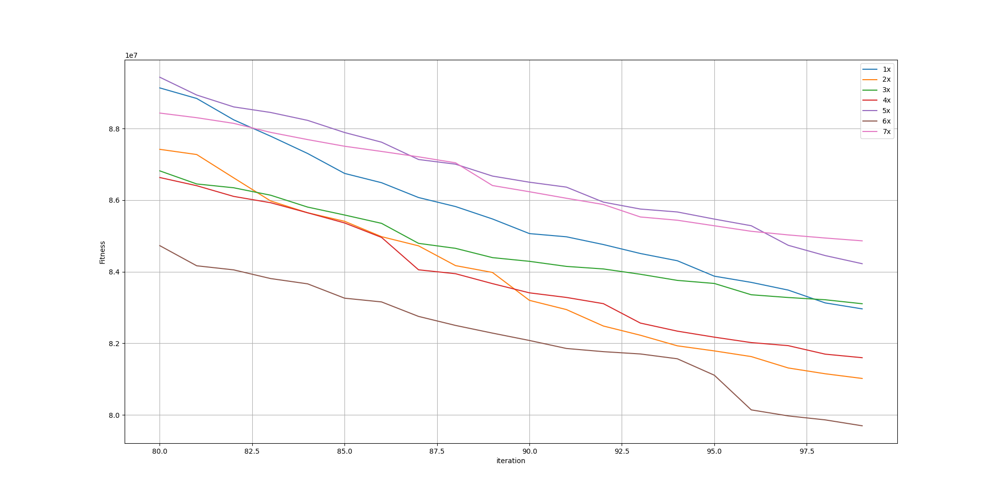
We can observe the spike happening when adding the cost of unpainted pixels is flattening as the maximum size of a brush stroke increase. And looking further in more details for the last iterations, we can observe the fitnesses aren’t that different:
To put it into context, let’s look at the original picture, followed by paintings with brush sizes of 1x, 2x and 7x:
|
|
 |
 |
While we can see they are all pretty close, we can observe the areas of low gradients are even less detailed the higher the maximum size of a brush. On the other hand, we can observe better details for the high gradient areas such as the center of the flower. However my favorite is the painting with the maximum brush size of 2x as the higher ones tend to leave too much detail out of the low gradient areas.
This makes sense as smaller maximum brush sizes force the painting to use more strokes to depict the very same area. And larger maximum brush sizes enable the painting to spend more strokes in areas where the fitness would reward it better, which are typically areas with more gradient. Thus picking a maximum brush size too large would result in a painting with uneven depictions, which may not be pleasant to the human eye, even if they do have similar fitness.
Conclusion
It’s a very interesting topic, in which one could go very deep. It’s also full of nuances and arbitrary decisions, especially when it comes to the aesthetics qualities of the resulting paintings.
Further work
Here are some ideas I would love to explore further at some point:
- Other methods to compare paintings with the original picture
- Use a prompt and a critic rather than a picture as a target
- incorporate the gradient sampling method into the fitness method
- Finding the sweet spot between an artistic painting and something closer to a photography. I do have more paintings with different level of iterations and have selected the best ones manually. However it would be interesting to think about some metric or fitness function I could use
- I have used the same set of brushes since the beginning. It would be nice to upgrade them or explore entirely new styles of brushes
- I have used a very simple way to simulate brush strokes. However there are a few non photorealistic methods that could enhance the results
- Exploring more approaches to guide the attention. It would help remediate the issues observed when the brushes where at 7x their normal size