Mixture Models on GPU
Preface
The purpose of this document is to serve me as notes and is not meant to be taken as exhaustive or a fully fledged blog post.
Introduction
Mixture models are a probabilistic view of the data, by decomposing it across different probility distributions.
In this example, we will use a Genetic Algorithm based approach for the detemination of the best mixture of probility distributions for a set of 2D points. We will focus on normal distributions only. As we are looking at a potentially large set of items, doing such computation on CPU may take too much time. Thus we will also look at doing these computations on a GPU and the associated challenges.
Solving that challenge means we will need a few things:
- We need to generate a dataset that we can cluster
- We need to figure out a good way to represent our population of clusters, which are our solutions
- We need to establish a way to grade our clusters, which is our fitness evaluation function
- We will also have to configure our evolution with some sensible policies for selection, combination and mutation
- We will need to modify our algorithms so they can be run on a GPU and interface with them
What is a Mixture Model?
As the name implies, it assumes the data is generated from a model \$ccM\$ of a mixture of k probability distributions. This can be expressed as:
\$f^"point"(bar X_j|ccM) = sum_{i=0}^{k-1}alpha_i*f^i(bar X_j)\$
with \$sum_{i=0}^{k-1}alpha_i = 1\$
Where:
- \$ccM\$ represents the whole model, ie. the combination of these mixture components
- \$bar X_j\$ represents the \$j^{th}\$ data point out of the \$j in {1...n}\$ points in the dataset
- \$alpha_i\$ represents the prior probability for a given component
- \$f^i(bar X_j)\$ is the \$i^{th}\$ probability density function
Then if we generalize it to a dataset \$ccD\$ of points \$bar X_0...bar X_{n-1}\$, the probability density of this data being generated by that model \$ccM\$ is the product of probability density of each of these points:
\$f^{data}(ccD|ccM) = prod_{j=0}^{n-1}f^{"point"}(bar X_j|ccM)\$
The goal will then be about finding the model \$ccM\$ which explains the best the dataset \$ccD\$, and thus maximizes \$f^{data}(ccD|ccM)\$. However it is often easier to optimize for \$log(f^{data}(ccD|ccM))\$ since it transforms the product into a sum and reduces possible underflow and overflows computations.
This means we will now try to optimize:
\$log(f^{data}(ccD|ccM)) = sum_{j=0}^{n-1}log(f^{"point"}(bar X_j|ccM)) \$
Effectively, this means our Genetic Algorithm will explore populations of various number of distributions and parameters and derive their fitness based on how high their \$log(f^{data}(ccD|ccM))\$ is. There will be some interesting challenges as we strive to find the inviduals which explain the most data with the least amount of distributions.
Project setup
In order to do our clustering, we do need a dataset. To that end, we will generate multiple groups of 2D points.
The dataset is generated by first generating some random centroids and leveraging Apache Commons Math to generate some samples:
final int maxPossibleDistributions = MAX_NUM_DISTRIBUTIONS - 1;
logger.info("Generating dataset");
final int numDistributions = randomGenerator.nextInt(MIN_NUM_DISTRIBUTIONS, MAX_NUM_DISTRIBUTIONS);
logger.info("Generating {} distributions:", numDistributions);
final double[][] means = new double[numDistributions][2];
final double[][][] covariances = new double[numDistributions][2][2];
final int[] cluster = new int[NUM_POINTS_PER_DISTRIBUTION * numDistributions];
final float[][] samples = new float[NUM_POINTS_PER_DISTRIBUTION * numDistributions][2];
final double[][] samplesDouble = new double[NUM_POINTS_PER_DISTRIBUTION * numDistributions][2];
for (int i = 0; i < numDistributions; i++) {
means[i] = new double[] { randomGenerator.nextDouble(MIN_MEAN, MAX_MEAN),
randomGenerator.nextDouble(MIN_MEAN, MAX_MEAN) };
/**
* See
* https://stackoverflow.com/questions/619335/a-simple-algorithm-for-generating-positive-semidefinite-matrices
*/
final double[][] randomMatrix = new double[][] {
{ randomGenerator.nextDouble(0, 4) - 2, randomGenerator.nextDouble(0, 4) - 2 },
{ randomGenerator.nextDouble(0, 4) - 2, randomGenerator.nextDouble(0, 4) - 2 } };
final double[][] covariance = new double[][] {
{ randomMatrix[0][0] * randomMatrix[0][0] + randomMatrix[0][1] * randomMatrix[0][1],
randomMatrix[0][0] * randomMatrix[1][0] + randomMatrix[0][1] * randomMatrix[1][1] },
{ randomMatrix[0][0] * randomMatrix[1][0] + randomMatrix[0][1] * randomMatrix[1][1],
randomMatrix[1][0] * randomMatrix[1][0] + randomMatrix[1][1] * randomMatrix[1][1] } };
covariances[i] = covariance;
logger.info("\t index: {} - mean: {} - covariance: {}", i, means[i], covariance);
final var multivariateNormalDistribution = new MultivariateNormalDistribution(means[i], covariance);
for (int j = 0; j < 5; j++) {
final var sample = multivariateNormalDistribution.sample();
logger.info("\t\t{} - {}", sample, multivariateNormalDistribution.density(sample));
}
for (int j = 0; j < NUM_POINTS_PER_DISTRIBUTION; j++) {
final var sample = multivariateNormalDistribution.sample();
samples[i * NUM_POINTS_PER_DISTRIBUTION + j] = new float[] { (float) sample[0], (float) sample[1] };
samplesDouble[i * NUM_POINTS_PER_DISTRIBUTION + j] = sample;
cluster[i * NUM_POINTS_PER_DISTRIBUTION + j] = i;
}
}
final float[] x = new float[NUM_POINTS_PER_DISTRIBUTION * numDistributions];
final float[] y = new float[NUM_POINTS_PER_DISTRIBUTION * numDistributions];
for (int i = 0; i < NUM_POINTS_PER_DISTRIBUTION * numDistributions; i++) {
x[i] = samples[i][0];
y[i] = samples[i][1];
}
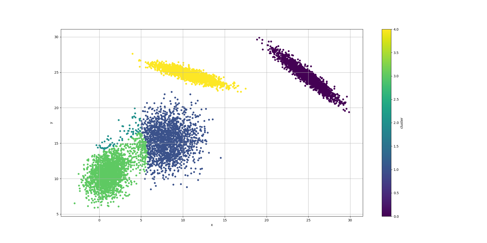
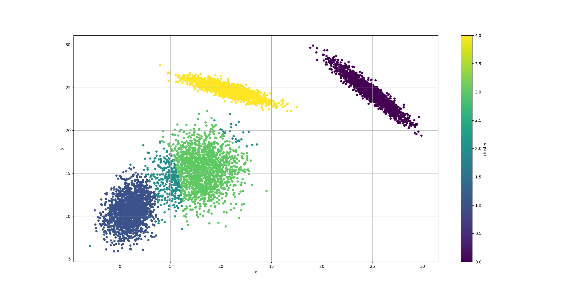
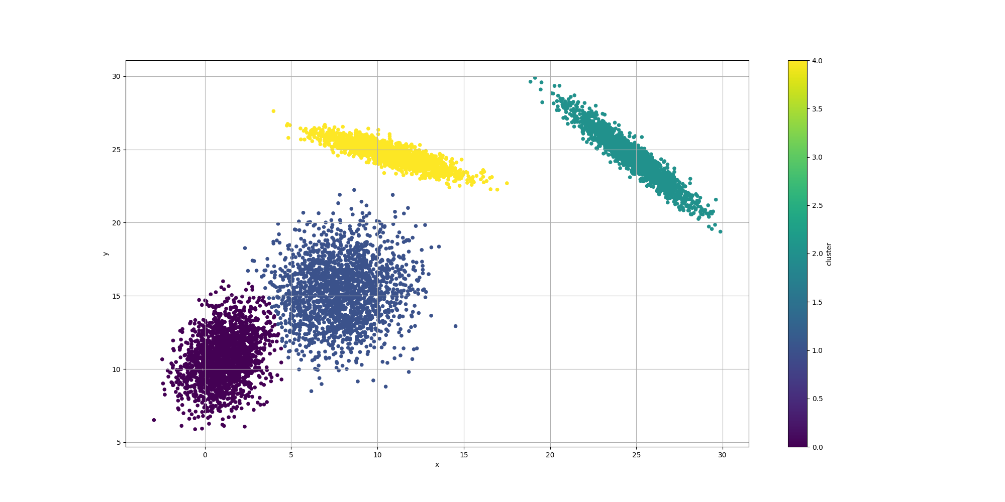
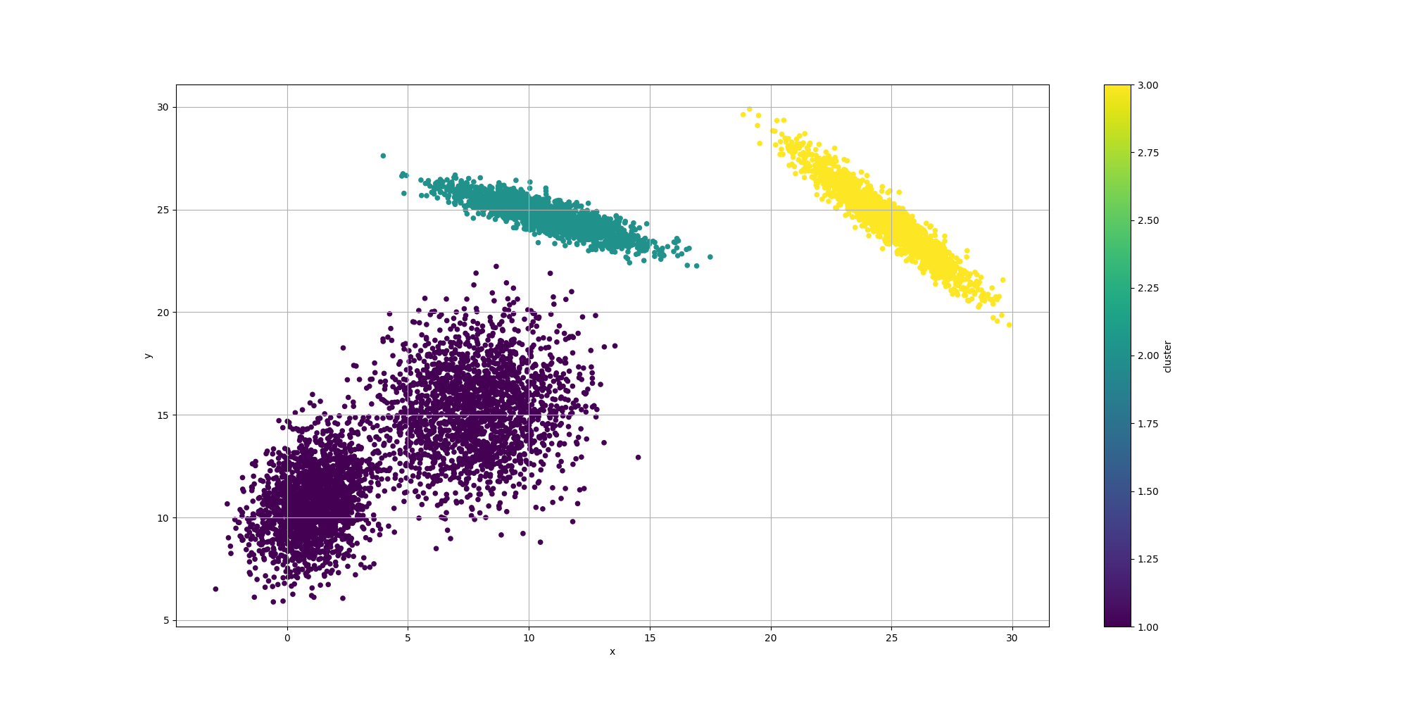
ClusteringUtils.persistClusters(x, y, cluster, baseDir + "original.csv");Here is how the resulting data would look like:
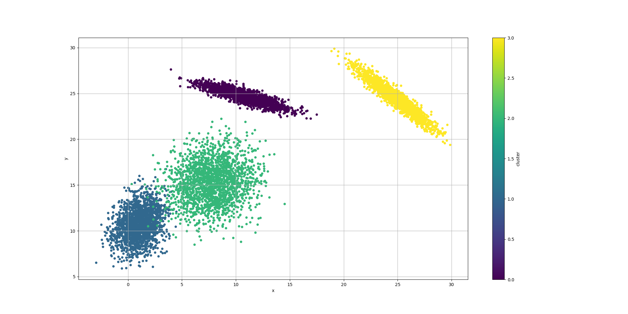
Note how some of the clusters are really close to each others and somewhat overlapping. This will have an impact in the way the algorithms decide to cluster them and it will be interesting to observe how each algorithm decides to approach that ambiguity.
Baseline - Expectation-Maximization
We want to compare our results with the ones produced by the most popular algorithm to estimate the parameters of a mixture model: Expectation-Maximization. As it is pretty similar to K-means, it suffers from the same issue converging towards a local optimum, and not necessarily the global optimum.
Apache Commons Math provide such support and we will use it to compute our baseline:
logger.info("Evaluating with commons math");
final var mmmmm = new MultivariateNormalMixtureExpectationMaximization(samplesDouble);
final var initialEstimatedDistribution = MultivariateNormalMixtureExpectationMaximization
.estimate(samplesDouble, numDistributions);
mmmmm.fit(initialEstimatedDistribution);
final var mixtureMultivariateNormalDistribution = mmmmm.getFittedModel();
final var components = mixtureMultivariateNormalDistribution.getComponents();
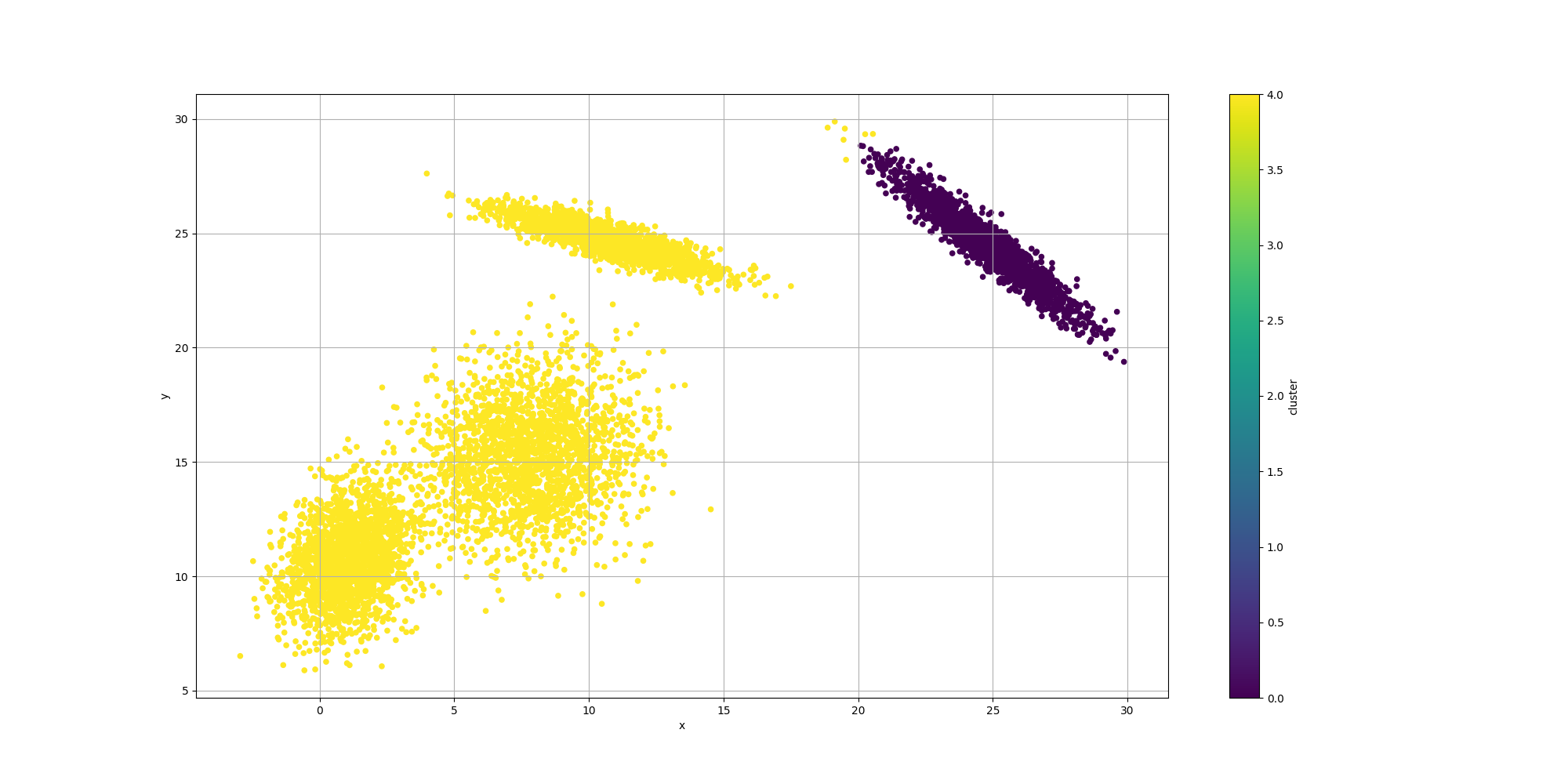
final var fittedCommonsMathGenotype = toGenotype(maxPossibleDistributions, mixtureMultivariateNormalDistribution);Here is the output of such execution:
Evolutionary Algorithm
Representation
If we expand the function we want to optimize for, we can write:
\$log(f^{data}(ccD|ccM)) = sum_{j=0}^{n-1}log(f^{"point"}(bar X_j|ccM)) = sum_{j=0}^{n-1}log(sum_{i=0}^{k-1}alpha_i*f^i(bar X_j))\$
And since we are limiting ourselves to mixtures composed of Normal distributions, we can assume:
\$f^i(bar X_j) = 1/(2*pi*sqrt(|Sigma|))e^(-1/2*(x-mu)^T*Sigma^-1*(x-mu))\$
Where:
- \$mu\$ is the mean vector for that distribution
- \$Sigma\$ is the covariance matrix \$[[sigma_x,sigma_(xy)],[sigma_(xy),sigma_y]]\$
This means we will nave n mixtures and each one will require a total of 6 pieces of information:
- \$alpha_i\$ which is a scalar
- \$mu\$ which is a 2d vector
- \$Sigma\$ which is the covariance matrix. Since the covariance matrix for a normal distribution is a symmetric positive semi-definite matrix, we will only require three elements \$sigma_x, sigma_y, sigma_(xy)\$
- \$|Sigma|\$ is the determinant of the covariance matrix
- \$Sigma^-1\$ is the inverse of the covariance matrix
As a result, we will use a DoubleChromosomeSpec or FloatChromosomeSpec with values ranging 0 to 30, which is the range of the generated distributions. We will add an extra translation step for the covariances since their values could also be negative.
Alternatively, we could have use values between 0 and 1 and apply translation and scaling as appropriate.
First attempt - Single Objective Method
Since our genotype describes a model with the mixtures and their parameter, the fitness function can bluntly compute \$log(f^{data}(ccD|ccM))\$. Since it is a double, the genetic algorithm will try to optimize that and we should end up with some interesting results. Here is the definition of fitness function:
public Fitness<Double> fitnessCPU(final int numDistributions, final double[][] samples) {
        return genotype -> {
                final var fChromosome = genotype.getChromosome(0, DoubleChromosome.class);

                /**
                 * Normalize alpha
                 */
                double sumAlpha = 0.0F;
                int k = 0;
                while (k < fChromosome.getSize()) {
                        sumAlpha += fChromosome.getAllele(k);
                        k += distributionNumParameters;
                }

                double[] likelyhoods = new double[samples.length];
                int i = 0;
                while (i < fChromosome.getSize()) {

                        final double alpha = fChromosome.getAllele(i) / sumAlpha;
                        if (alpha > 0.0001) {
                                final double[] mean = new double[] { fChromosome.getAllele(i + 1), fChromosome.getAllele(i + 2) };
                                final double[][] covariances = new double[][] {
                                                { fChromosome.getAllele(i + 3) - 15, fChromosome.getAllele(i + 4) - 15 },
                                                { fChromosome.getAllele(i + 4) - 15, fChromosome.getAllele(i + 5) - 15 } };

                                try {
                                        final var multivariateNormalDistribution = new MultivariateNormalDistribution(mean, covariances);

                                        for (int j = 0; j < samples.length; j++) {
                                                final var density = multivariateNormalDistribution.density(samples[j]);
                                                likelyhoods[j] += alpha * density;
                                        }
                                } catch (NonPositiveDefiniteMatrixException | MathUnsupportedOperationException
                                                | SingularMatrixException e) {
                                        // Ignore invalid mixtures
                                }
                        }
                        i += distributionNumParameters;
                }

                double sumLogs = 0.0F;
                for (int j = 0; j < samples.length; j++) {
                        sumLogs += Math.log(likelyhoods[j]);
                }

                return sumLogs / samples.length;
        };
}
Note it may be tempting to use a Silhouette score like we did in Clustering, but that would not too well since our mixtures aren’t globular and thus could not fit well. However that’s because we were using an euclidian distance. It may be interesting to investigate the use of the Silhouette score in conjunction with a Mahalanobis distance, which would be appropriate if the underlying distributions are assumed to be gaussian.
With regards to the configuration of the genetic algorithm, we will use a combination of creep, random and swap mutations, which will help explore the search space along with looking for better values.
The code for the configuration is:
final Builder<Double> eaConfigurationBuilder = new EAConfiguration.Builder<>();
eaConfigurationBuilder
                .chromosomeSpecs(DoubleChromosomeSpec.of(distributionNumParameters * maxPossibleDistributions, 0, 30))
                .parentSelectionPolicy(Tournament.of(2))
                .combinationPolicy(
                                MultiCombinations.of(
                                                SinglePointArithmetic.of(0.9),
                                                        SinglePointCrossover.build(),
                                                        MultiPointCrossover.of(2),
                                                        MultiPointArithmetic.of(2, 0.9)))
                .mutationPolicies(
                                MultiMutations.of(
                                                RandomMutation.of(0.40),
                                                        CreepMutation.of(0.40, NormalDistribution.of(0.0, 2)),
                                                        SwapMutation.of(0.30, 5, false)))
                .fitness(fitnessCPU(maxPossibleDistributions, samples))
                .termination(Terminations.ofMaxGeneration(maxGenerations));

if (CollectionUtils.isNotEmpty(seedPopulation)) {
        eaConfigurationBuilder.seedPopulation(seedPopulation);
}

final var eaConfiguration = eaConfigurationBuilder.build();
The execution context is also straightforward with a population of 250 individuals:
final var csvEvolutionListener = CSVEvolutionListener.<Double, Void>of(
                baseDir + "mixturemodel-so-cpu.csv",
                        List.of(
                                        ColumnExtractor.of("generation", e -> e.generation()),
                                                ColumnExtractor.of("fitness", e -> e.fitness())));

final var eaExecutionContextBuilder = EAExecutionContexts.<Double>standard();
eaExecutionContextBuilder.populationSize(250)
                .addEvolutionListeners(csvEvolutionListener, EvolutionListeners.ofLogTopN(logger, 5))
                .build();
final var eaExecutionContext = eaExecutionContextBuilder.build();
Results
Here is an example of evolution of the fitness over time:
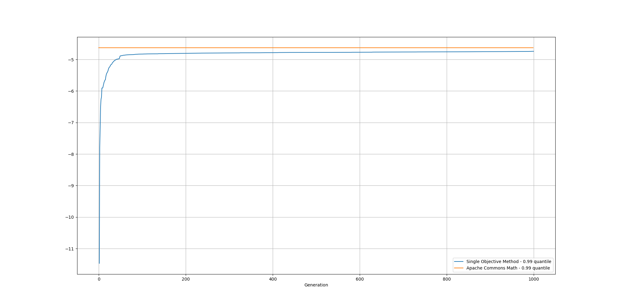
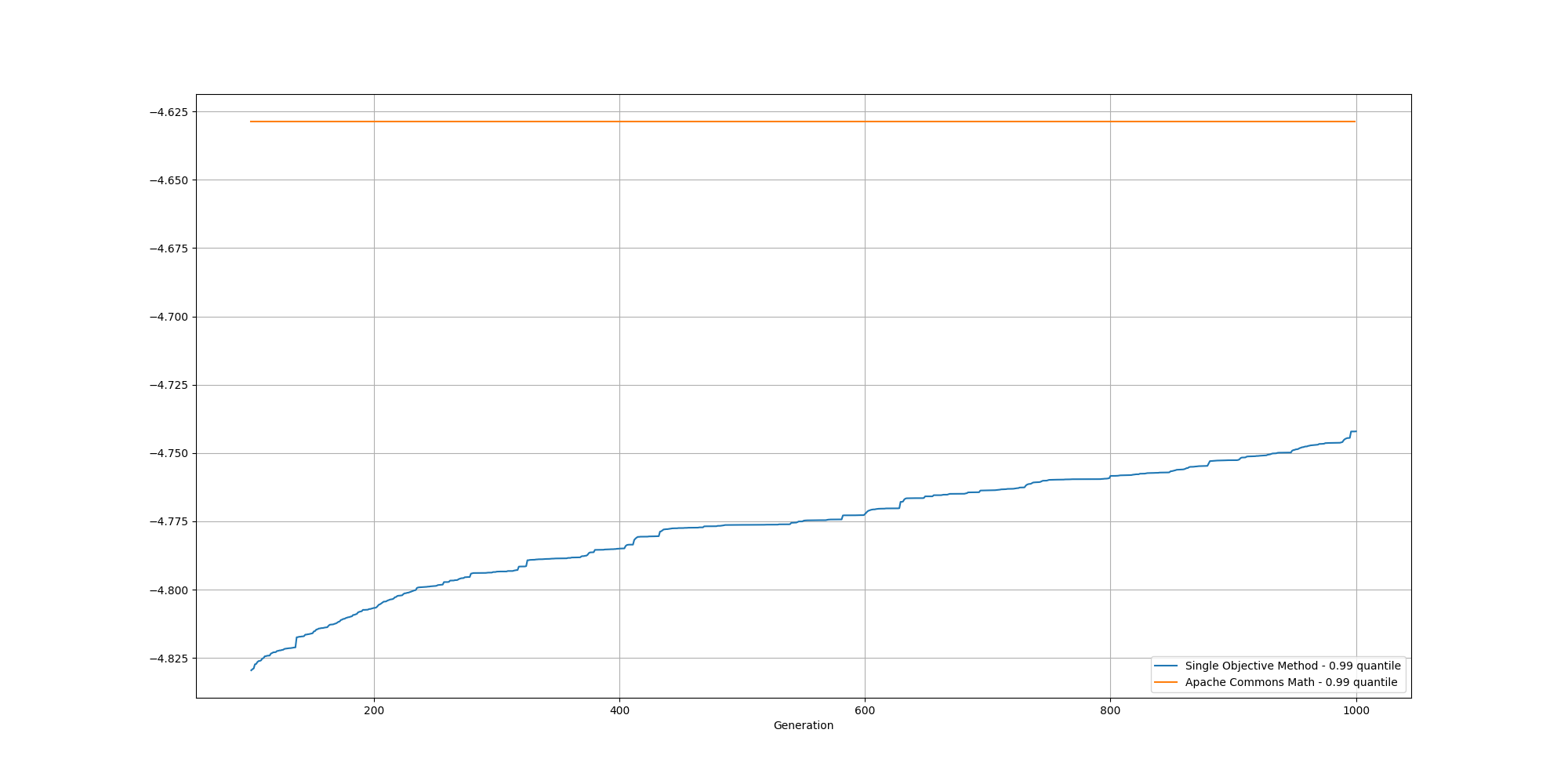
And if we cut off the first 100 generations, we can better observe the slow increase and could reasonably expect it to reach the same or better score than the baseline with enough generations:
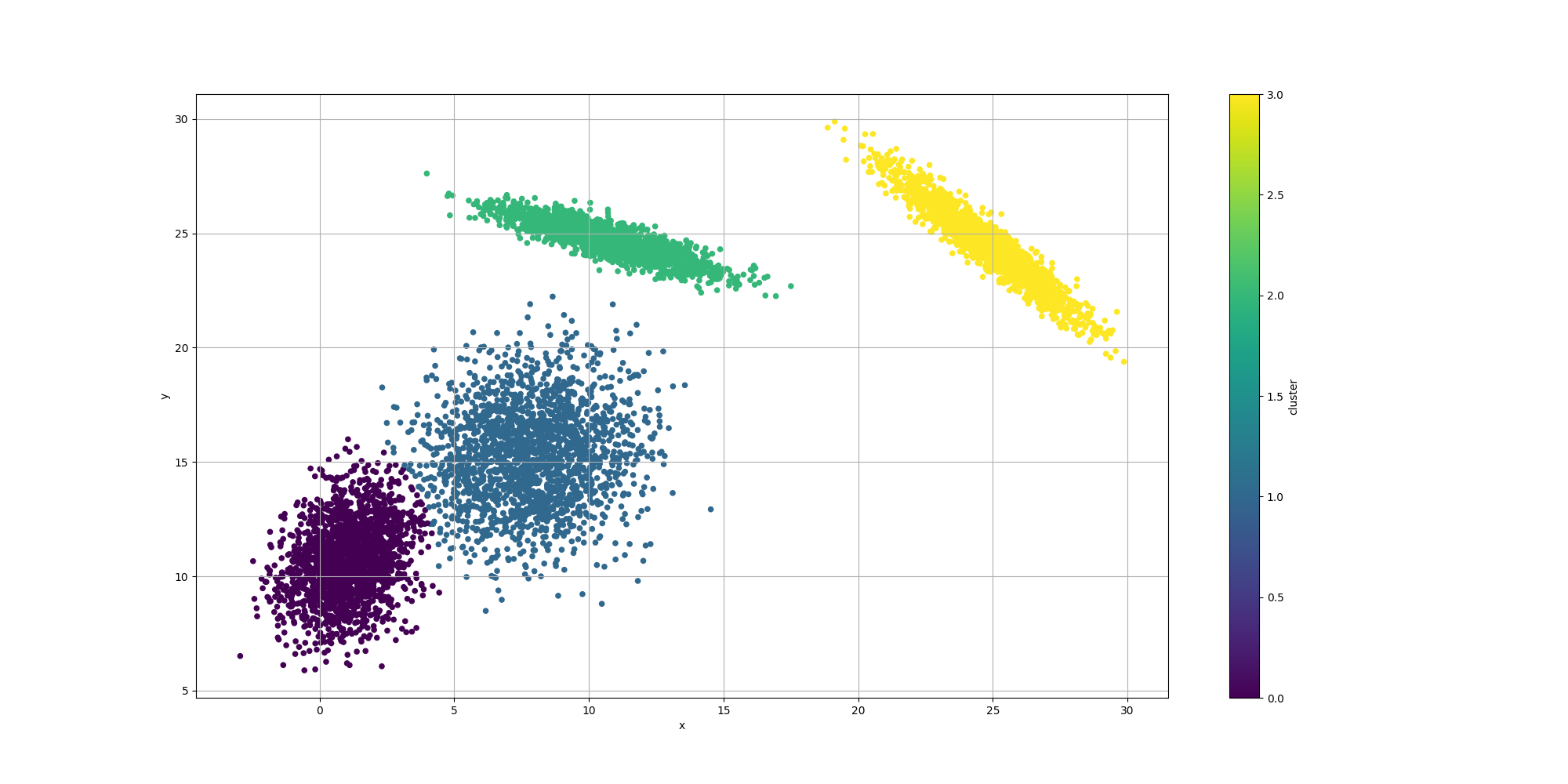
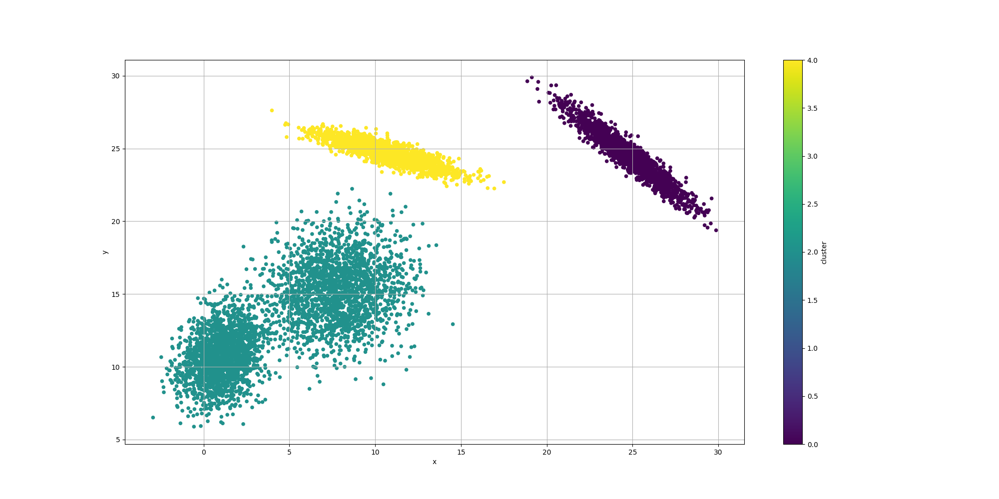
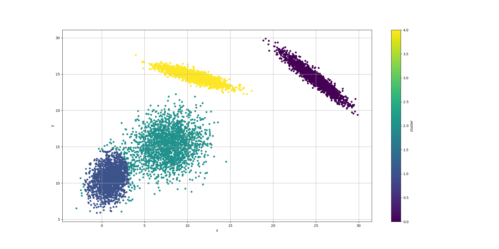
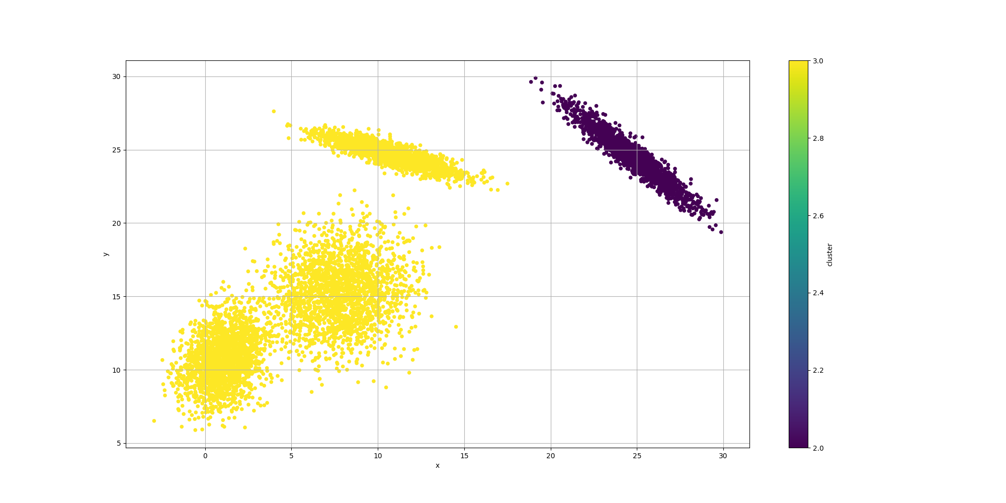
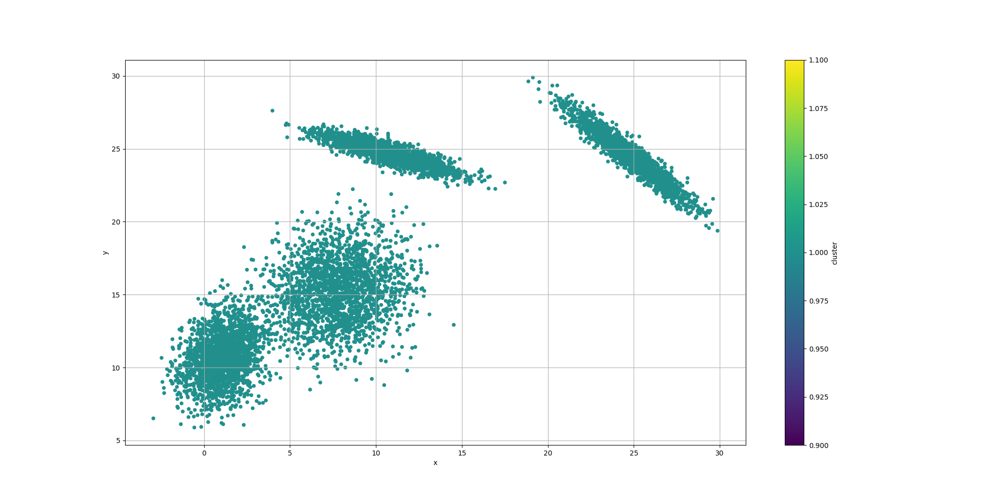
With regards to the clustering itself, while the clusters are pretty well defined, we do observe some surprising results for the centroids:
We observe the clustering looks overall reasonable, except for the lower left where there appears to be an extra cluster and the boundaries look a bit off. It would be interesting to weigh in the impact of the number of clusters. We could look at AIC or BIC which incorporate the complexity of the model with its likelihood. However let’s try to evaluate them separately.
Second attempt - Multi Objective Optimization
One way to look at the problem is that there is a tradeof between the best fit and the number of clusters. So we could translate it in a multi objective optimization problem where we can express such trade off.
The fitness function would now return a vector with two components:
- The likelihood of such model, as in the previous section
- The number of unused clusters
The fitness function would be pretty similar to the previous one:
public Fitness<FitnessVector<Float>> fitnessCPU(final int numDistributions, final double[][] samples) {
        return genotype -> {
                final var fChromosome = genotype.getChromosome(0, FloatChromosome.class);

                float sumAlpha = 0.0F;
                int k = 0;
                while (k < fChromosome.getSize()) {
                        final float alpha = fChromosome.getAllele(k);
                        sumAlpha += alpha;

                        k += distributionNumParameters;
                }

                float[] likelyhoods = new float[samples.length];
                int i = 0;
                while (i < fChromosome.getSize()) {

                        final float alpha = fChromosome.getAllele(i) / sumAlpha;
                        if (alpha > 0.0001) {
                                final double[] mean = new double[] { fChromosome.getAllele(i + 1), fChromosome.getAllele(i + 2) };
                                final double[][] covariances = new double[][] {
                                                { fChromosome.getAllele(i + 3) - 15, fChromosome.getAllele(i + 4) - 15 },
                                                { fChromosome.getAllele(i + 4) - 15, fChromosome.getAllele(i + 5) - 15 } };

                                try {
                                        final var multivariateNormalDistribution = new MultivariateNormalDistribution(mean, covariances);

                                        for (int j = 0; j < samples.length; j++) {
                                                final var density = multivariateNormalDistribution.density(samples[j]);
                                                likelyhoods[j] += alpha * density;
                                        }
                                } catch (NonPositiveDefiniteMatrixException | MathUnsupportedOperationException
                                                | SingularMatrixException e) {
                                }
                        }
                        i += distributionNumParameters;
                }

                float sumLogs = 0.0F;
                for (int j = 0; j < samples.length; j++) {
                        sumLogs += Math.log(likelyhoods[j]);
                }

                final int[] assigned = ClusteringUtils
                                .assignClustersFloatChromosome(distributionNumParameters, samples, genotype);
                final Set<Integer> uniqueAssigned = new HashSet<>();
                uniqueAssigned.addAll(IntStream.of(assigned).boxed().toList());

                final float numUnusedCluster = uniqueAssigned.isEmpty() ? -10f
                                : (float) (numDistributions - uniqueAssigned.size());

                return new FitnessVector<>(sumLogs / samples.length, numUnusedCluster);
        };
}
With regards to the configuration, except for the NSGA2 part, it is pretty much the same:
final var fitnessFunc = fitnessCPU(maxPossibleDistributions, samples);

final Builder<FitnessVector<Float>> eaConfigurationBuilder = new EAConfiguration.Builder<>();
eaConfigurationBuilder
                .chromosomeSpecs(FloatChromosomeSpec.of(distributionNumParameters * maxPossibleDistributions, 0, 30))
                .parentSelectionPolicy(TournamentNSGA2Selection.ofFitnessVector(2, 3, deduplicator))
                .replacementStrategy(
                                Elitism.builder()
                                                .offspringRatio(0.950)
                                                .offspringSelectionPolicy(TournamentNSGA2Selection.ofFitnessVector(2, 3, deduplicator))
                                                .survivorSelectionPolicy(NSGA2Selection.ofFitnessVector(2, deduplicator))
                                                .build())
                .combinationPolicy(
                                MultiCombinations.of(
                                                SinglePointArithmetic.of(0.9),
                                                        SinglePointCrossover.build(),
                                                        MultiPointCrossover.of(2),
                                                        MultiPointArithmetic.of(2, 0.9)))
                .mutationPolicies(
                                MultiMutations.of(
                                                RandomMutation.of(0.40),
                                                        CreepMutation.of(0.40, NormalDistribution.of(0.0, 1)),
                                                        SwapMutation.of(0.40, 5, false)))
                .fitness(fitnessFunc)
                .termination(Terminations.ofMaxGeneration(maxGenerations));

if (CollectionUtils.isNotEmpty(seedPopulation)) {
        eaConfigurationBuilder.seedPopulation(seedPopulation);
}

final var eaConfiguration = eaConfigurationBuilder.build();
And the same can be said about its execution context:
final var csvEvolutionListener = CSVEvolutionListener.<FitnessVector<Float>, Void>of(
                baseDir + "mixturemodel-moo-cpu.csv",
                        List.of(
                                        ColumnExtractor.of("generation", e -> e.generation()),
                                                ColumnExtractor.of("fitness", e -> e.fitness().get(0)),
                                                ColumnExtractor.of("numUnusedCluster", e -> e.fitness().get(1))));

final var eaExecutionContextBuilder = EAExecutionContexts.<FitnessVector<Float>>standard();
eaExecutionContextBuilder.populationSize(250)
                .addEvolutionListeners(
                                csvEvolutionListener,
                                        EvolutionListeners.<FitnessVector<Float>>ofLogTopN(
                                                        logger,
                                                                5,
                                                                Comparator.<FitnessVector<Float>, Float>comparing(fv -> fv.get(0))))
                .build();
final var eaExecutionContext = eaExecutionContextBuilder.build();
Results
Let’s look at the results for the best likelyhood across the number of clusters:

If we look at the overall fitness, we can observe a similar behavior than before:
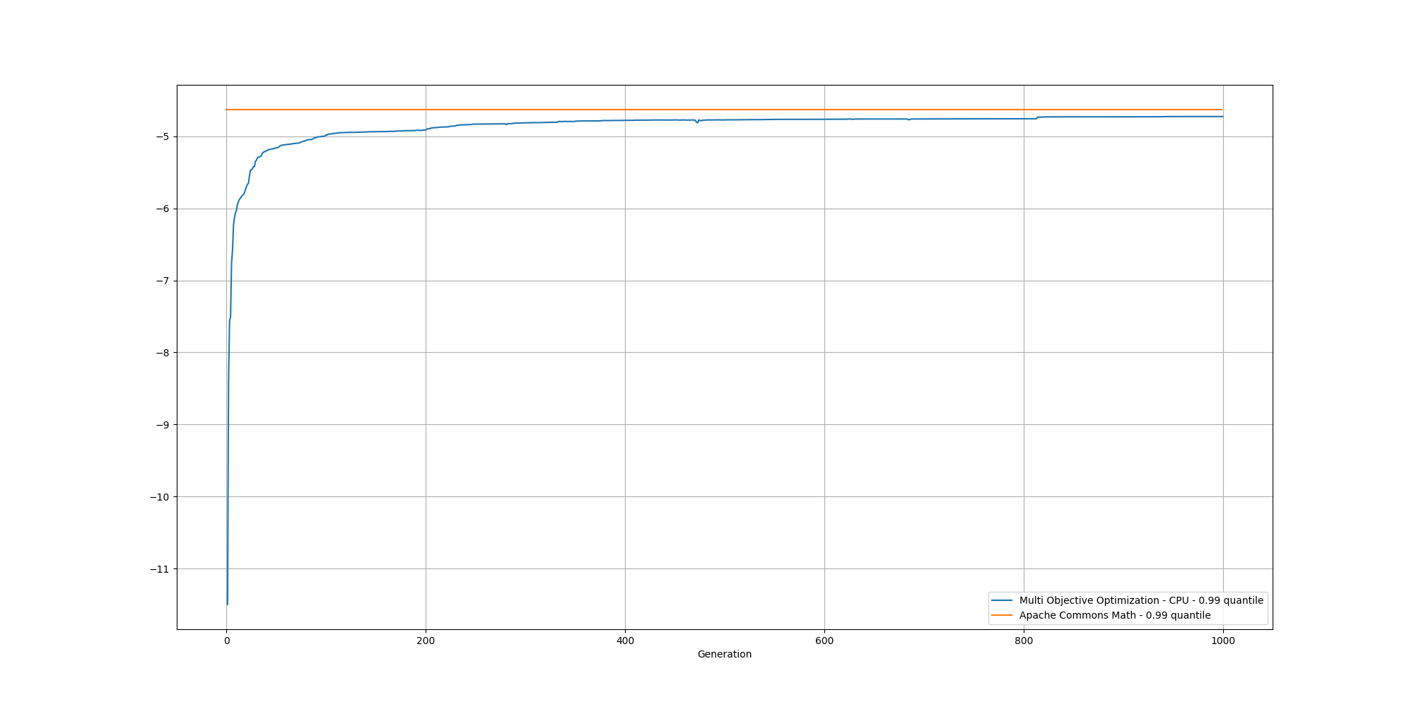
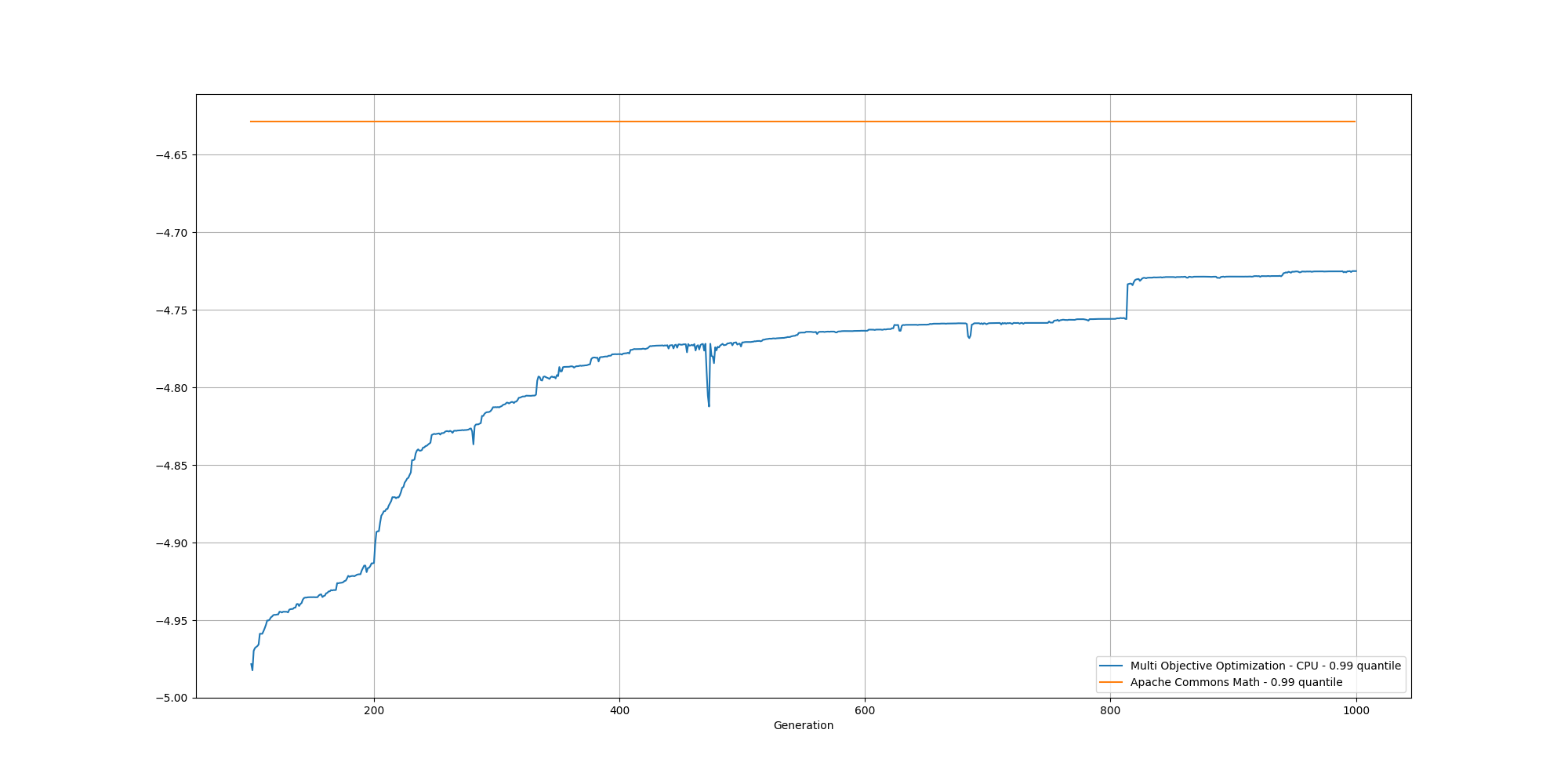
And if we cut off the first 100 generations, we can better observe the slow increase and could reasonably expect it to reach the same or better score than the baseline with enough generations:
This looks great, however it does take some time to compute. In order to accelerate the process, let’s now look at accelerating this with the help of a GPU
Third attempt - Multi Objective Optimization over GPU
Leveraging GPUs can be quite a daunting task as they can be complex to interact with. Fortunately, Genetics4j does provide a few facilities to make it easier and safer to use OpenCL for hardware acceleration. Let’s go through a cursory review of them.
GPUEAConfiguration
First, let’s observe the configuration itself has not changed much comparing to the previous approaches:
final var singleKernelFitness = SingleKernelFitness
                .of(singleKernelFitnessDescriptor, fitnessExtractor(maxPossibleDistributions, samplesDouble));

final var eaConfigurationBuilder = GPUEAConfiguration.<FitnessVector<Float>>builder()
                .chromosomeSpecs(FloatChromosomeSpec.of(chromosomeSize, 0, 30))
                .parentSelectionPolicy(TournamentNSGA2Selection.ofFitnessVector(2, 5, deduplicator))
                .replacementStrategy(
                                Elitism.builder()
                                                .offspringRatio(0.950)
                                                .offspringSelectionPolicy(TournamentNSGA2Selection.ofFitnessVector(2, 5, deduplicator))
                                                .survivorSelectionPolicy(NSGA2Selection.ofFitnessVector(2, deduplicator))
                                                .build())
                .combinationPolicy(
                                MultiCombinations.of(
                                                SinglePointArithmetic.of(0.9),
                                                        SinglePointCrossover.build(),
                                                        MultiPointCrossover.of(3),
                                                        MultiPointArithmetic.of(3, 0.9)))
                .mutationPolicies(
                                MultiMutations.of(
                                                RandomMutation.of(0.40),
                                                        CreepMutation.of(0.40, NormalDistribution.of(0.0, 1)),
                                                        SwapMutation.of(0.40, 5, false)))
                .program(Program.ofResource("/opencl/mixturemodel/main.cl", kernelName, ""))
                .fitness(singleKernelFitness)
                .termination(Terminations.ofMaxGeneration(maxGenerations));

if (CollectionUtils.isNotEmpty(seedPopulation)) {
        eaConfigurationBuilder.seedPopulation(seedPopulation);
}

final var eaConfiguration = eaConfigurationBuilder.build();
The main differences we can observe are:
- We are now using GPUEAConfiguration instead of a EAConfiguration
- We have a new program definition to inform Genetics4j
- There is a new way to specify how to define the fitness
SingleKernelFitness is a way to specify two things:
- SingleKernelFitnessDescriptor - How to call the OpenCL clusters, including some contextual information such as the work size as well as the parameters to pass to said kernel
- FitnessExtractor - How to massage the result of the execution of the kernel into the actual fitness metric
SingleKernelFitnessDescriptor
Here is how we use it:
final var singleKernelFitnessDescriptorBuilder = SingleKernelFitnessDescriptor.builder();
singleKernelFitnessDescriptorBuilder.kernelName(kernelName)
                .kernelExecutionContextComputer(KernelExecutionContextComputers.ofGlobalWorkSize1D(samples.length))
                .putStaticDataLoaders(0, StaticDataLoaders.ofLinearize(samples))
                .putStaticDataLoaders(
                                1,
                                        StaticDataLoaders
                                                        .of(distributionNumParameters, maxPossibleDistributions, chromosomeSize, samples.length))
                .putDataLoaders(2, DataLoaders.ofGenerationAndPopulationSize())
                .putDataLoaders(3, DataLoaders.ofLinearizeFloatChromosome(0))
                .putDataLoaders(4, DataLoaders.ofFloatSupplier(computeSideData(maxPossibleDistributions)))
                .putResultAllocators(5, ResultAllocators.ofMultiplePopulationSizeFloat(samples.length));
final var singleKernelFitnessDescriptor = singleKernelFitnessDescriptorBuilder.build();
We can observe it specifies a few information with regards to which kernel to execute and how, but also how to prepare the parameters and data to pass to the kernel. There are actually four types of parameters Genetics4j offers in its abstraction:
- Static data, which is data that never changes across the genotype and generation. This is helpful to specify some side data or global parameters
- Dynamic data, which can depend on the specific genotypes and generation. This may contains the population, some related metadata or the result of some population specific computation
- Local memory, which can be used as temporary buffers for the computations done on the GPU
- Result allocators, which are buffers allocated to store the results and compute the final fitness score
Fitness Extractor
Here is how we define it:
public final FitnessExtractor<FitnessVector<Float>> fitnessExtractor(final int maxPossibleDistributions,
                final double[][] samples) {
        return (openCLExecutionContext, kernelExecutionContext, executorService, generation, genotypes,
                        resultExtractor) -> {

                final float[] results = resultExtractor.extractFloatArray(openCLExecutionContext, 5);

                try {
                        final var extractionTask = executorService.submit(() -> {
                                return IntStream.range(0, genotypes.size()).boxed().parallel().map(genotypeIndex -> {
                                        float tally = 0;

                                        final int startIndex = genotypeIndex * samples.length;
                                        final int endIndex = startIndex + samples.length;
                                        int notFiniteCount = 0;
                                        for (int i = startIndex; i < endIndex; i++) {
                                                if (Float.isFinite(results[i])) {
                                                        tally += results[i];
                                                } else {
                                                        notFiniteCount++;
                                                        tally -= 10_000f;
                                                }
                                        }
                                        final int[] assignedClusters = ClusteringUtils.assignClustersFloatChromosome(
                                                        distributionNumParameters,
                                                                samples,
                                                                genotypes.get(genotypeIndex));
                                        final Set<Integer> uniqueAssigned = new HashSet<>();
                                        uniqueAssigned.addAll(IntStream.of(assignedClusters).boxed().toList());

                                        if (notFiniteCount > 0 || notFiniteCount == samples.length || uniqueAssigned.isEmpty()) {
                                                return new FitnessVector<>(-100_000_000f, -100f);
                                        }

                                        final float numUnusedCluster = (float) (maxPossibleDistributions - uniqueAssigned.size());
                                        return new FitnessVector<>(tally / samples.length, numUnusedCluster);
                                }).toList();
                        });

                        return extractionTask.get();
                } catch (InterruptedException | ExecutionException e) {
                        logger.error("Could not extract results", e);
                        throw new RuntimeException(e);
                }
        };
}
The interesting part is how we use the resultExtractor to extract the results of the OpenCL kernel to transform it into a FitnessVector<Float>>.
GPUEAExecutionContext
Here is how we define it:
final var csvEvolutionListener = CSVEvolutionListener.<FitnessVector<Float>, Void>of(
                baseDir + algorithmName + ".csv",
                        List.of(
                                        ColumnExtractor.of("generation", e -> e.generation()),
                                                ColumnExtractor.of("fitness", e -> e.fitness().get(0)),
                                                ColumnExtractor.of("numUnusedCluster", e -> e.fitness().get(1)),
                                                ColumnExtractor.of("numCluster", e -> maxPossibleDistributions - e.fitness().get(1))));

final var topNloggerEvolutionListener = EvolutionListeners.<FitnessVector<Float>>ofLogTopN(
                logger,
                        5,
                        Comparator.<FitnessVector<Float>, Float>comparing(fv -> fv.get(0)));

final var eaExecutionContextBuilder = GPUEAExecutionContext.<FitnessVector<Float>>builder()
                .deviceFilters(DeviceFilters.ofGPU())
                .populationSize(250)
                .addEvolutionListeners(csvEvolutionListener, topNloggerEvolutionListener);

/**
 * TODO should be in the library
 */
eaExecutionContextBuilder.addSelectionPolicyHandlerFactories(
                gsd -> new NSGA2SelectionPolicyHandler<>(),
                        gsd -> new TournamentNSGA2SelectionPolicyHandler<>(gsd.randomGenerator()));

eaExecutionContextBuilder.addReplacementStrategyHandlerFactories(gsd -> new SPEA2ReplacementStrategyHandler<>());

final var eaExecutionContext = eaExecutionContextBuilder.build();
It is used in the very same way than a regular EAExecutionContext, except for additional helpers to finely control which device(s) are to be used. The evolution will take advantage of all the selected devices, significantly increasing the computation speed in the case of multiple GPUs or hardware accelerators.
Results
Looking at the logs, we can confirm Genetics4j is leveraging all the GPUs devices it could find on the machine:
01:23:31.936 DEBUG n.b.g.g.GPUFitnessEvaluator - Genotype decomposed in 2 partition(s)
01:23:31.948 DEBUG n.b.g.g.s.f.SingleKernelFitness - Intel(R) Graphics [0x9a60] - Took 33.047 microsec for 250 genotypes
01:23:31.975 DEBUG n.b.g.g.s.f.SingleKernelFitness - NVIDIA GeForce RTX 3060 Laptop GPU - Took 1366.255 microsec for 250 genotypes
The increased execution speed means we can run algorithms on larger populations, for larger dataset and for far more generations!
Then let’s look at the results for the best likelyhood across the number of clusters:


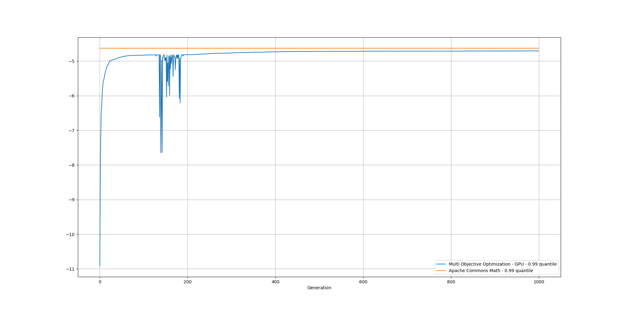
If we look at the overall fitness, we can observe a similar behavior than before:
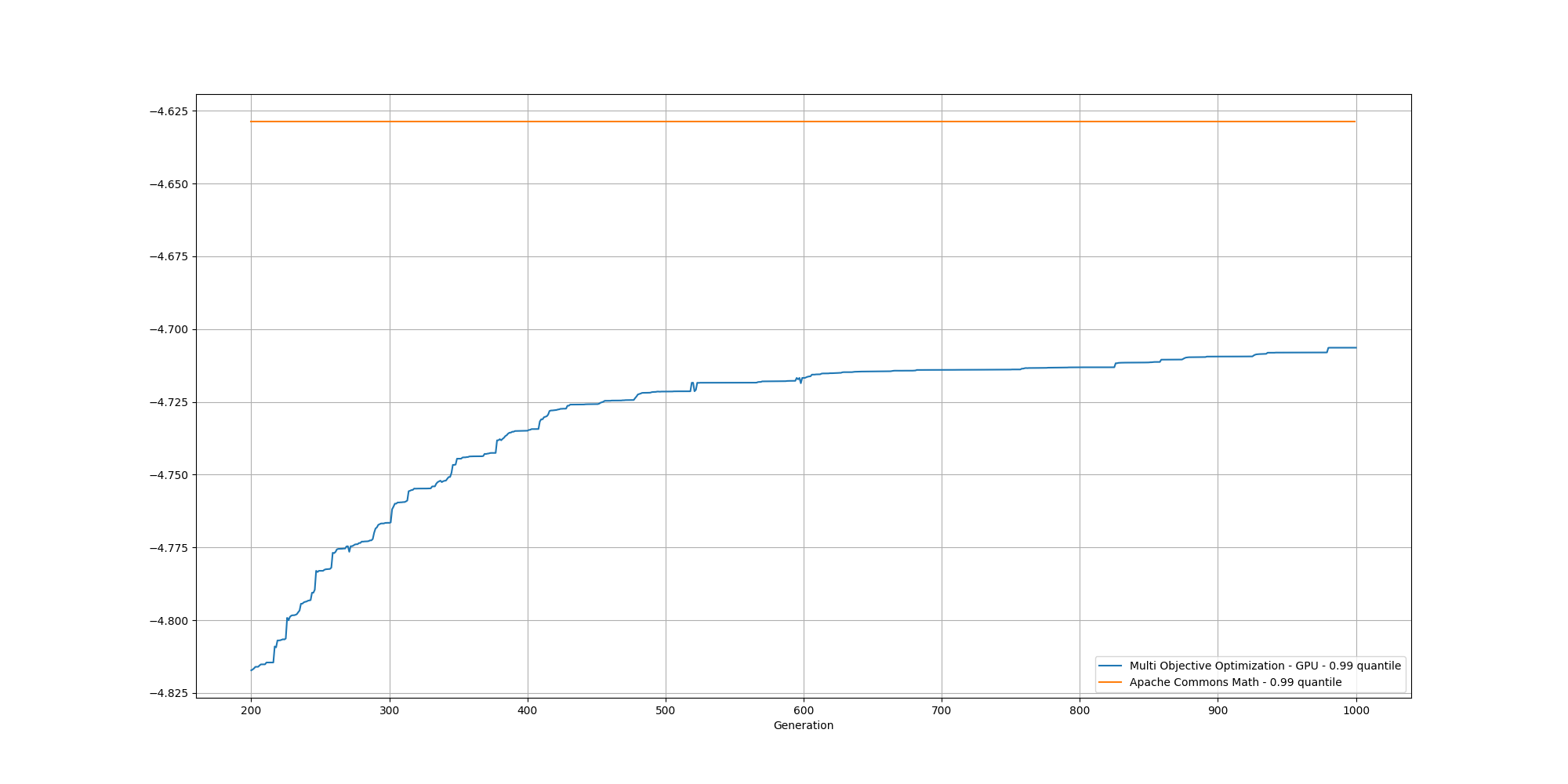
And if we cut off the first 200 generations, we can better observe the slow increase and could reasonably expect it to reach the same or better score than the baseline with enough generations:
Fourth attempt - Multi Objective Optimization with seed over GPU
Over the past few attempts, we have observed the Expectation-Maximization approach can yield quite good results in a short time but also that the Genetic Algorithm approach can explore many more potential solutions, especially thanks to the help of GPUs. So why not combining both?
To do so, we need to pass the mixtures found by the Expectation-Maximization model as a seed individual of the Genetic Algorithm, which will use it as part of its initial population. This can be done using this parameter from EAConfiguration:
eaConfigurationBuilder.seedPopulation(seedPopulation);Results
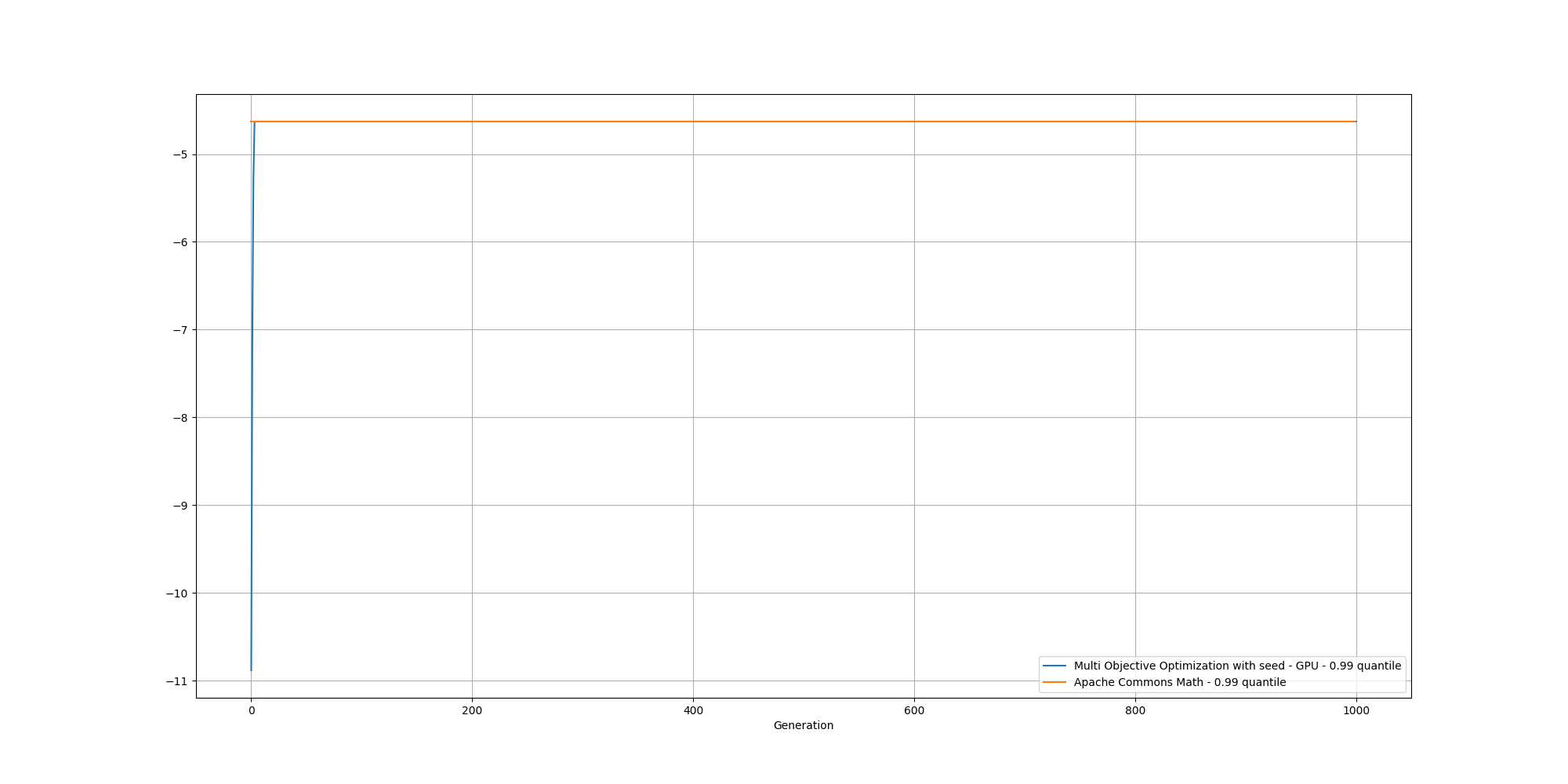
Then let’s look at the results for the best likelyhood across the number of clusters:

If we look at the overall fitness, we can observe a similar behavior than before:
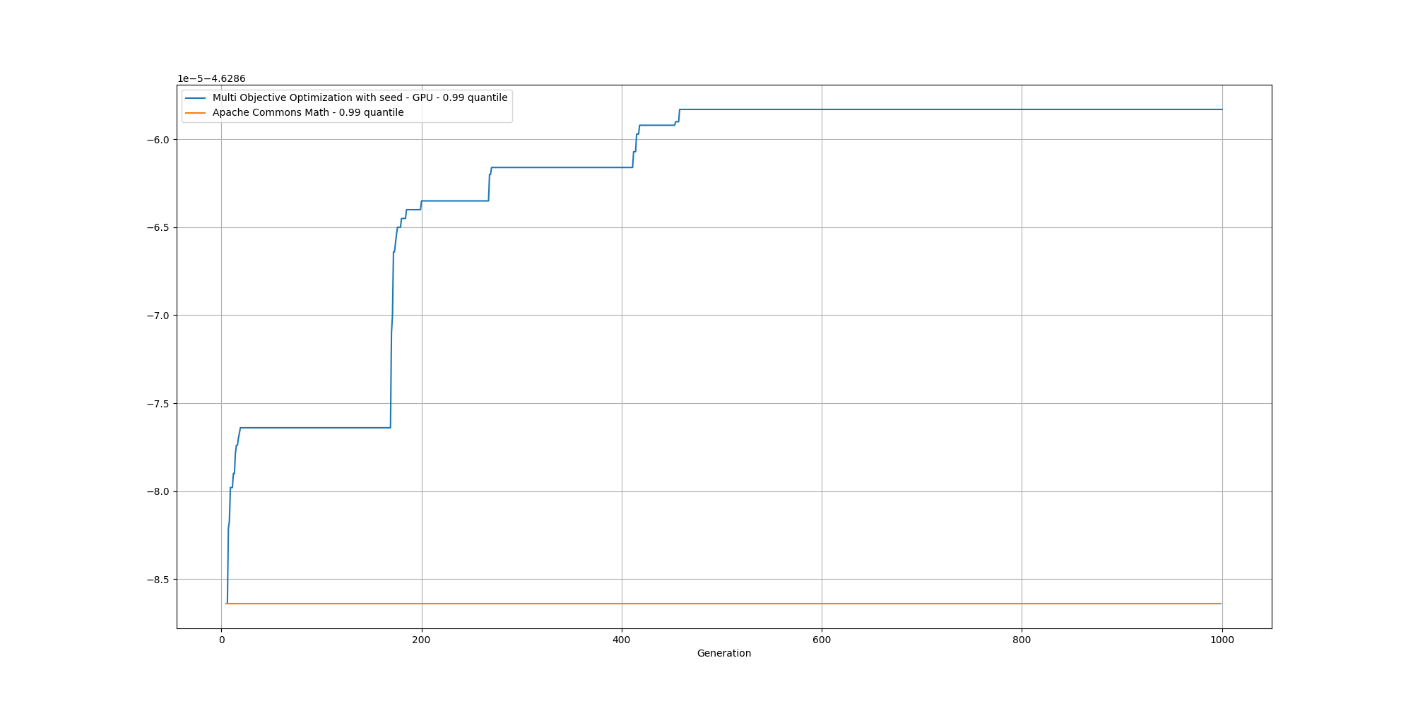
And if we cut off the first few generations to get a better view, we can observe the fitness improving upon the baseline pretty quickly:
Conclusion
Genetic Algorithms can be pretty effective at clustering data without making some assumption about the underlying dataset. This can be especially be useful in more complex scenario. We also observe that the increase in parameters will also increase the time to find more acceptable solution as the solution space is much larger.
Leveraging GPUs, we are also able to work on more complex challenges in a more reasonable time, enabling faster iterations and broader exploration of the solution space.
Furthermore, combining both classical approaches such as Expectation-Maximization and Genetic Algorithm have enabled us to get some reasonable solutions pretty quickly while potentially avoiding local maxima.
Going further
This is a rather simple example but there are tons of room for improvement.
- We have not looked at incorporating AIC or BIC into the scoring methodology
- The way we compute the fitness score is far from being optimized, whether the CPU version or the GPU one
- Instead of assuming centroids have a specific location, we could consider them instead as statistical distributions and thus a Mixture model
- We have not explored Fitness Sharing
- We have focused on normal distributions. But it would be fun to explore the combination of different types of distributions