NEAT Streaming Parity Classification
Introduction

Streaming parity classification is about receiving a sequence of bits and computing the parity bit, which tells us if there was an even or odd number of 1 seen in that input sequence. In this article, I will focus on 4-bit long sequences.
The network receives an infinite stream of bits but only has access to the current bit at a given timestep, so the running context must live inside the recurrent state.
It highlights the situations where NEAT must lean on a RecurrentNetwork.
Code overview
The evaluator feeds one input bit plus a bias into the network at each timestep. The network has to output whether the prefix observed so far contains an odd (1) or even (-1) number of ones. Purely feed-forward NEAT networks cannot solve the task because they forget the history once a timestep is processed. Thus the need for a recurrent neural network.
This means we expect a recurrent network with two inputs and one output. The two inputs are composed of the current bit in the sequence along with a bias input and the output is the expected parity bit given the sequence seen so far.
Training dataset
We generate 100 sequences of randomly chosen 4 bit sequences.
private static final List<List<Integer>> TRAINING_SEQUENCES = random.ints(100)
                .mapToObj(i -> random.doubles(4).mapToInt(j -> j <= 0.5 ? 0 : 1).boxed().toList())
                .toList();
We could wonder about the biases types of examples generated this way, but that will be for another time.
Fitness
The sequences are encoded as -1 / 1 inputs to match the tanh activation. After each timestep, the output is
compared with the expected parity and the absolute error is accumulated for all sequences. The maximum score equals \$"number of bits" * "range(-1,1)" * "number of sequences"\$, ensuring a maximum fitness that is high enough to push the population toward consistent predictions.
And let’s not forget to reset the state of the network between each sequence to ensure independent results.
private Fitness<Float> createParityFitness(final boolean verbose) {
        return genotype -> {
                final NeatChromosome chromosome = genotype.getChromosome(0, NeatChromosome.class);

                if (chromosome.getConnections().isEmpty()) {
                        return 0f;
                }

                final RecurrentNetwork network = buildNetwork(chromosome);
                final Integer outputNodeIndex = chromosome.getOutputNodeIds().getFirst();

                float cumulativeError = 0F;
                for (final List<Integer> sequence : TRAINING_SEQUENCES) {
                        network.resetState();

                        Map<Integer, Float> outputs = Map.of();
                        List<Integer> input = new ArrayList<>(4);
                        for (final int bit : sequence) {
                                input.add(bit);
                                final float expectedValue = expectedParity(input);

                                outputs = network.step(Map.of(0, encodeBit(bit), 1, 1.0f));

                                final float prediction = outputs.getOrDefault(outputNodeIndex, 0.0f);
                                final float error = Math.abs(expectedValue - prediction);
                                cumulativeError += error;

                                if (verbose) {
                                        logger.info("Sequence {} -> expected {}, predicted {}", input, expectedValue, prediction);
                                }
                        }

                }

                return MAX_THEORETICAL_FITNESS - cumulativeError;
        };
}
Configuration
Overview
private EAConfiguration<Float> buildParityConfiguration(final List<MutationPolicy> mutations) {
        Objects.requireNonNull(mutations);

        final Builder<Float> builder = new EAConfiguration.Builder<>();
        builder.chromosomeSpecs(NeatChromosomeSpec.of(2, 1, -3, 3))
                        .parentSelectionPolicy(buildSelectionPolicy())
                        .combinationPolicy(NeatCombination.build())
                        .mutationPolicies(mutations)
                        .fitness(createParityFitness(false))
                        .optimization(Optimization.MAXIMIZE)
                        .termination(
                                        Terminations.<Float>or(
                                                        Terminations.ofMaxTime(Duration.ofMinutes(5)),
                                                                Terminations.ofStableFitness(200),
                                                                Terminations.ofMaxGeneration(2000),
                                                                Terminations.ofFitnessAtLeast(FITNESS_TERMINATION_THRESHOLD)));
        return builder.build();
}
The configuration mirrors standard NEAT problems. We define a single NEAT chromosome with selection, combination and mutation. We also ensure tight termination conditions via perfect score, which demonstrates we solved the problem, or a maximum set of duration, generations or inability to make progress.
Selection
Similalry, selection uses a pretty standard set of parameters:
private SelectionPolicy buildSelectionPolicy() {
        return NeatSelection.builder()
                        .minSpeciesSize(3)
                        .perSpeciesKeepRatio(0.20f)
                        .speciesSelection(Tournament.of(3))
                        .speciesPredicate(
                                        (i1, i2) -> NeatUtils.compatibilityDistance(i1.genotype(), i2.genotype(), 0, 2, 2, 1f) < 3)
                        .build();
}
Mutation
In terms of mutations, we will have 3 kinds of operators:
- Weight mutations, be it completely random new values or adjustments
- Structural changes by adding orremoving nodes and connections
- Switching the state of a connection
Given the nature of the problem we want to solve, we do require additional connections and thus we note the probability to add a connection is far higher than the probability to add a node.
The add-connection policy also allows output nodes as connection sources. This lets evolution create feedback from an output into a hidden node or another output, which the recurrent evaluator can propagate across its iterations.
final double randomWeightsProb = 0.05;
final double switchMutationProb = 0.005;
final double addNodeProb = 0.015;
final double deleteNodeProb = 0.005;
final double addConnectionProb = 0.035;
final double deleteConnectionProb = 0.005;
private List<MutationPolicy> buildMutations(final double randomWeightsProb, final double switchMutationProb,
final double addNodeProb, final double deleteNodeProb, final double addConnectionProb,
final double deleteConnectionProb) {
return List.of(
RandomMutation.of(randomWeightsProb),
MultiMutations.of(
CreepMutation.of(0.85f, NormalDistribution.of(0.0, 0.333)),
NeatConnectionWeight.builder().populationMutationProbability(0.85f).build()),
SwitchStateMutation.of(switchMutationProb),
AddNode.of(addNodeProb),
DeleteNode.of(deleteNodeProb),
AddConnection.builder()
.populationMutationProbability(addConnectionProb)
.allowOutputNodeAsSource(true)
.build(),
DeleteConnection.of(deleteConnectionProb));
}Overview
Let’s look at an example of generated solution but I also want to take a look at the impact of the parameters.
Here is an example of generated solution:

As a reminder, dashed lines mean the connection is disabled. We can see quite a few nodes with connections disabled or that lead to nowhere. They are all remnants of the exploration done. After simplifying the network, it looks like:

We can note this looks much simple now and that both nodes 4 and 6 have backlinks in this network.
At first, I was exploring only computing the parity bit for the final bit once the sequence was seen, and most solutions involved a single backlink. This is an interesting contrast where I do observe two backlinks in most solutions where it needs to compute the parity bit at all steps of the bit sequence.
Number of nodes vs connections
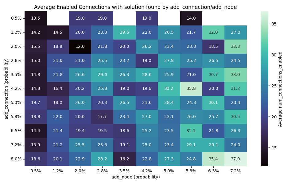
I wanted to explore the impact of nodes comparing to connections.
So I have have done 10 runs for each combination of values for the add connection/node mutation and here are the results
Solution founds
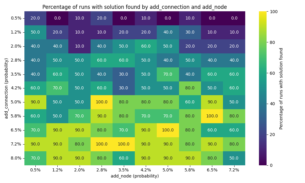
We can see that the number of connection has far more impact than the number of nodes. I would actually go as far as saying the number of note doesn’t really impact the results here.
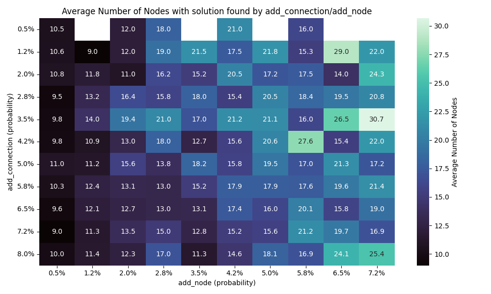
Runtime
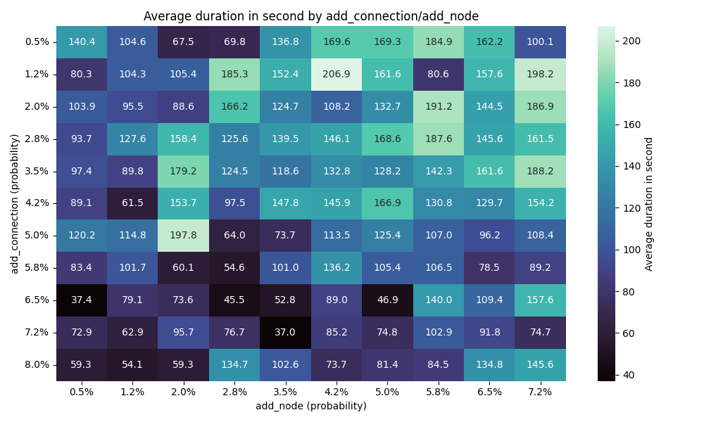
This chart makes sense as the addition of connections makes it faster to find a solution, and having more nodes would require more exploration.
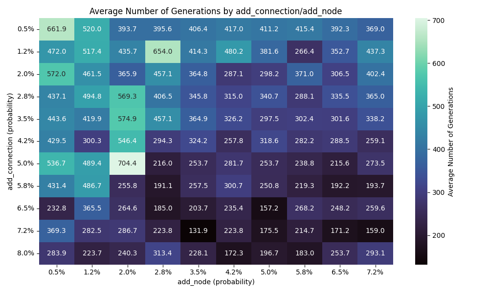
Here, the more nodes and connections, the less generation required to find a solution
Future ideas
- Exploring the impact of the crowding function as it will carve out the niches to explore
- Plotting the number and quality of the niches over time
- Exploring combining NEAT with MOO by having a fitness function combining the current fitness and also the size of the network. We could then observe the pareto front of the best solution given the complexity of the network
- I have focused on 4 bit streams, but what about longer sequences? How does that impact the amount of work to find solutions?
- Would our current network trained on 4 bit streams work on longer streams? I would expect it to decay over time, but how far would that be?
- What if we used Gated Recurrent Unit ? They can be quite useful to create a stable memory and help us in this scenario